DB2 Server for VSE & VM Application Programming (Version 7 Release 5)

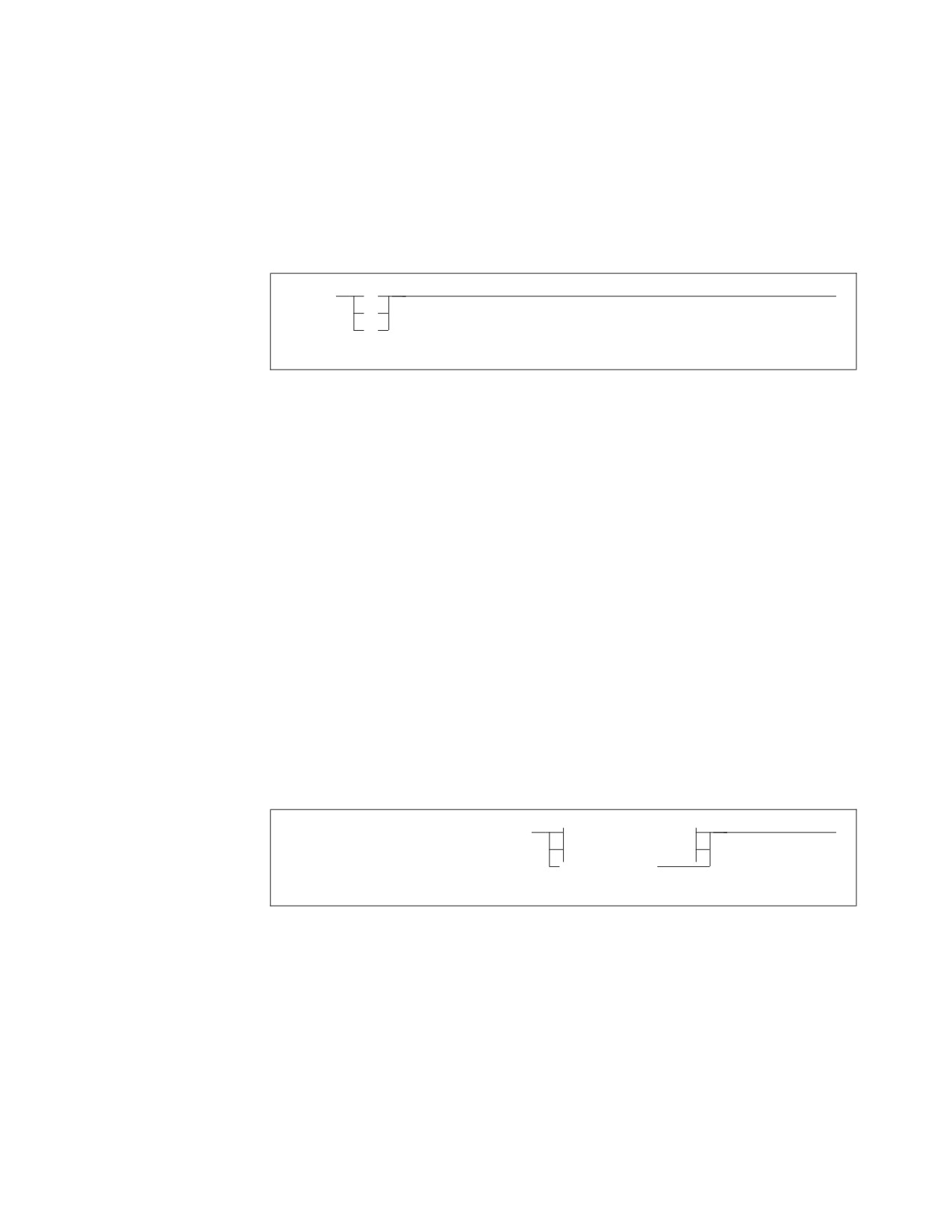
Using the WITH Clause

The WITH clause specifies the isolation level for the query, which overrides any

other isolation level specification. For example, a statement specifying WITH UR in

a package prepped with ISOL(CS) will use an isolation level of uncommitted read.

For more information on isolation levels, see “Selecting the Isolation Level to Lock

Data” on page 134 (DB2 Server for VM) or “Selecting the Isolation Level to Lock

Data” on page 172 (DB2 Server for VSE).

►► WITH

►◄

Figure 15. Format of the WITH clause

Retrieving or Inserting Multiple Rows

Using the Cursor with a Select-Statement

The previous section showed how to use a select-statement to create an SQL query.

You can now use that query to retrieve values into an application program from

multiple rows in a table.

To do so, you must first declare an SQL cursor, which is a control structure that

points to a row in a table. The rows returned by the query are called the result table

of the cursor.

A cursor can be in an open or a closed state. In the open state, it maintains a

position in its result table on a certain row (called the current row). If you delete the

current row, the cursor will be positioned between the two rows that surrounded

the deleted rows. If you request the next row and receive a message that there are

no more rows (SQLCODE 100 and SQLSTATE '02000'), the cursor will be

positioned after the last row. Before you OPEN the cursor, it is said to be

positioned before the first row.

Declaring a Cursor

►► DECLARE cursor_name CURSOR FOR

select-statement

►◄

insert-statement

statement_name

Figure 16. Format of the DECLARE CURSOR statement

Use the DECLARE CURSOR statement to define a cursor. This statement associates

a cursor_name with a specified select-statement, insert-statement, or statement-name.

For example:

DECLARE C1 CURSOR FOR SELECT LASTNAME, FIRSTNME

FROM EMPLOYEE WHERE SALARY>:AMT

DECLARE C2 CURSOR FOR INSERT INTO ACTIVITY

(ACTNO, ACTKWD, ACTDESC)

VALUES (:ACT, :KEYWORD, :DESC)

Chapter 3. Coding the Body of a Program

Note: Statement-name is only used with dynamic SQL. For an explanation of its

use, see “Retrieving the Query Result” on page 226.

The select-statement or insert-statement is a part of the DECLARE CURSOR

statement, so you must not place EXEC SQL in front of SELECT or INSERT

(however, do place it in front of the DECLARE).

Using a Cursor in an Application Program

Your program may contain many DECLARE CURSOR statements that define

different cursors and associate them with different queries. During the processing

of a program, several cursors may be in the open state at one time. It is possible to

define more than one cursor that operates on the same data within the same

logical unit of work. It is also possible to open a cursor and then operate on the

same data with a non-cursor operation such as a Searched DELETE. However,

mixing these operations should be avoided, because the result of one operation can

adversely affect another. For example, do not update a row using a Positioned

UPDATE and subsequently delete it with another cursor operation or with a

Searched DELETE.

The DECLARE CURSOR statement that defines a cursor must occur earlier in the

program than any statement operating on that cursor. It does not result in any

processing when the program is executed (that is, it does not automatically open

the cursor).

The scope of a cursor-definition is an entire program. Therefore, cursor names must

be unique within a program. You cannot have two DECLARE CURSOR statements

in the same program that use the same cursor-name, even if they are in different

blocks or procedures.

For additional detail on the DECLARE CURSOR statement, see the DB2 Server for

VSE & VM SQL Reference manual.

Manipulating the Cursor

After you define a cursor, you can manipulate it using the SQL statements shown

in Table 5. (See the DB2 Server for VSE & VM SQL Reference manual for a complete

description of these statements.)

Table 5. SQL Statements for Manipulating Cursors

Statements for

Manipulating Query and

Manipulating Query

Manipulating Insert

Insert Cursors

Cursors

OPEN

FETCH

PUT

Positioned DELETE

Positioned UPDATE

The OPEN Statement:

Partial Format:

►► OPEN cursor_name

►◄

If you are opening a query-cursor (a cursor defined in terms of a select-statement),

this statement examines the input host variables (if any) used in the definition of

Application Programming

the cursor, determines the result table for the cursor, and leaves it in the open

state. When the system executes an OPEN statement for a query-cursor, it positions

the cursor before the first row of the result table. After the query-cursor is opened,

the system does not reexamine its input variables until you close and reopen the

cursor. No rows in the result table are fetched to the host program until a FETCH

statement is executed. Always open the cursor before issuing the first FETCH or

PUT statement.

If you are opening an insert-cursor and your program is blocking, this statement

prepares the system to block the rows that are to be inserted. With an insert-cursor,

you can change the values of the input host variables between inserts; you do not

have to close and reopen the cursor.

The FETCH Statement:

Partial Format:

▼

►► FETCH cursor_name INTO

host_variable_list

►◄

This statement can be executed only when the indicated cursor is in the open state.

The position of the cursor is advanced to the next row of the result table, and the

selected columns of this row are delivered into the output host variables referenced

in the host_variable_list.

The following is an example of the FETCH statement:

DECLARE QUERY1 CURSOR FOR

SELECT EMPNO, BONUS*1.10

FROM EMPLOYEE

WHERE WORKDEPT='D11'

OPEN QUERY1

The values are

FETCH QUERY1 INTO :E1, :B1

returned in these

host variables.

A cursor can move forward only when it is in its result table; the system cannot

return to rows that have already been fetched (other than closing the cursor and

reopening it).

If the result table of the cursor is empty, or if all its rows have already been

fetched, the system returns the not found return code (SQLCODE=100 and

SQLSTATE='02000') and the cursor is positioned after the last row of the result

table. To perform further operations with the cursor, you must close and reopen it.

It is possible for two or more rows in the result table to have exactly the same

values. (For example, many rows of the EMPLOYEE table may have the same

WORKDEPT, and you might define a cursor that selects only WORKDEPT from

the table.) These duplicate values are not eliminated from the result table unless

you specify DISTINCT in the SELECT clause of the DECLARE CURSOR statement.

You can use indicator variables in the INTO clause. (For a detailed discussion of

indicator variables, see “Using Indicator Variables” on page 59.) Each main

variable in the INTO clause may, at your option, have an associated indicator

Chapter 3. Coding the Body of a Program

variable. If a null value is returned, and you haven’t provided an indicator

variable, a negative SQLCODE is returned to your program and execution of the

statement is halted.

The PUT Statement:

Partial Format:

►► PUT cursor_name

►◄

This statement can be executed only when the indicated cursor is in the open state.

The PUT statement inserts one row of data as defined by a cursor. The contents of

input host variables referenced in the host_variable_list (defined in the VALUES

clause of the DECLARE CURSOR statement for insert) are delivered to the

database.

For instance, the following statements insert a new row of data into the

EMPLOYEE table:

DECLARE CC CURSOR FOR

INSERT INTO EMPLOYEE (EMPNO, FIRSTNME, MIDINIT, LASTNAME, EDLEVEL)

VALUES (:EMP, :FIRST, :MID, :LAST, :ED)

OPEN CC

PUT CC

CLOSE CC

The values represented by the host variables :EMP, :FIRST, :MID, :LAST, and :ED

are placed into the corresponding columns of the new row. The other columns are

assigned the null value.

After the PUT statement is executed, you can assign different values to the input

host variables to add another row. Alternatively, you can place constants in the

VALUES clause of the DECLARE CURSOR statement instead of host variables.

This causes identical values to be inserted into the related columns for each PUT.

The PUT statement is used mostly for inserting multiple rows of data into a table

in groups or blocks (although, it also works with non-blocked inserts). Blocked

inserts are specified with the BLOCK preprocessor parameter. If blocking is in

effect, rows are not inserted until the block is full, or until a CLOSE statement is

issued. For information on preprocessing your program with the BLOCK option

specified, see “Preprocessing the Program” on page 114 (DB2 Server for VM) or

“Preprocessing the Program” on page 156 (DB2 Server for VSE). For information

on using the BLOCK option in DRDA protocol for DB2 Server for VM see “Using

the Blocking Option to Process Rows in Groups” on page 139.

The Positioned DELETE Statement:

Partial Format:

►► DELETE FROM table_name WHERE CURRENT OF cursor_name

►◄

This statement can be executed only when the indicated cursor is in the open state

and positioned on a row of the result table. It deletes that particular row from the

Application Programming

table. The cursor itself remains where it was; it is considered to be in the between

position and, cannot be used for further deletions or updates until it is

repositioned by a FETCH statement.

From the example under the FETCH statement, you could delete a row from the

EMPLOYEE table after doing a FETCH, by issuing:

DELETE FROM EMPLOYEE

WHERE CURRENT OF QUERY1

The Positioned UPDATE Statement:

Partial Format:

►► UPDATE table_name set_clause WHERE CURRENT OF cursor_name

►◄

This statement is similar to the DELETE statement, except that it updates the row

of the table on which the cursor is positioned rather than deleting it, leaving the

position of the cursor unchanged. When using this statement, you must specify the

update-clause in the select-statement.

The following example updates the SALARY column of each fetched row of the

EMPLOYEE table:

DECLARE QUERY2 CURSOR FOR

SELECT LASTNAME, FIRSTNAME, MIDINITT

FROM EMPLOYEE

WHERE WORKDEPT = 'D21'

FOR UPDATE OF SALARY

OPEN QUERY2

FETCH QUERY2 INTO :LAST, :FIRST, :MID

UPDATE EMPLOYEE

SET SALARY = SALARY + :DELTA

WHERE CURRENT OF QUERY2

CLOSE QUERY2

The CLOSE Statement:

Format:

►► CLOSE cursor_variable

►◄

The indicated cursor leaves the open state, and its result table becomes undefined.

No FETCH or PUT statement can be executed on the cursor, and no DELETE or

UPDATE statement can refer to its current position until the cursor is reopened by

an OPEN statement. The CLOSE statement permits the resources associated with

maintaining an open cursor to be released. It should be placed in your program so

that it is executed as soon as the program is finished using a cursor.

If your program is blocking, you can close an insert-cursor with an incomplete

block to insert the remaining rows.

Chapter 3. Coding the Body of a Program

Always close a cursor before committing changes. If changes are committed before

an insert cursor (that is being blocked) is closed, an error occurs.

Illustrating the Use of the Query Cursor

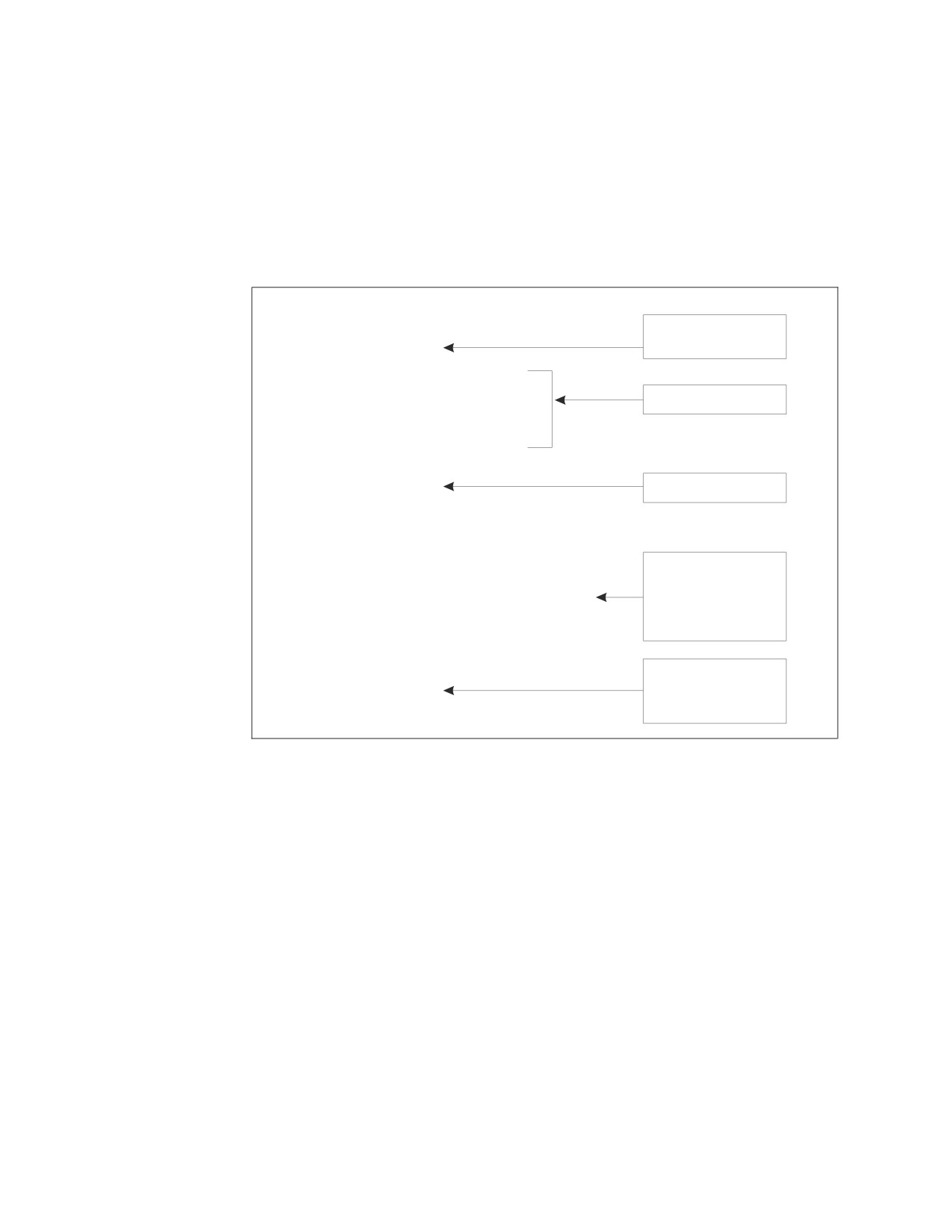
Figure 17, which shows a fragment of pseudocode, illustrates the use of a query

cursor C1. It finds the employees of all the rows of the EMPLOYEE table whose

department number matches host variable DEPT. The FETCH statements retrieve

the selected columns successively into host variables EMP, FNAME, and LNAME.

After the results are retrieved, they are displayed on the console.

Initialize DEPT (the

DEPT = ' D11'

input host variable).

EXEC SQL DECLARE C1 CURSOR FOR

SELECT EMPNO, FIRSTNME, LASTNAME

Declare cursor C1.

FROM EMPLOYEE

WHERE WORKDEPT=:DEPT

ORDER BY EMPNO

EXEC SQL OPEN C1

Open the cursor.

EXEC SQL FETCH C1 INTO :EMP, :FNAME, : LNAME

DO WHILE (SQLCODE=0)

Fetch the next row of

DISPLAY (EMP, FNAME, LNAME)

the result table into

EXEC SQL FETCH C1 INTO :EMP, :FNAME, :LNAME

the ouput host

END-DO

variables and display

them.

DISPLAY ('END OF LIST')

When the result table

EXEC SQL CLOSE C1

is empty, close the

cursor.

Figure 17. Using a Cursor

Recall that SQLCODE is set to +100 (SQLSTATE '02000') when there are no rows

remaining to be fetched.

Retrieving Single Rows

The SELECT INTO statement finds the only row of the table specified in the

FROM clause that satisfies the given search condition. From this row, the system

selects the columns that you supplied in the select-list. The results are inserted in

the host variables that you specified in the INTO clause. The data type and length

attributes of the host variables must be compatible with the data type and length

attributes of the expressions in the select-list. If specified, the WITH clause specifies

the isolation level to be used on the query and overrides any other isolation level

specification.

Application Programming

▼

►►

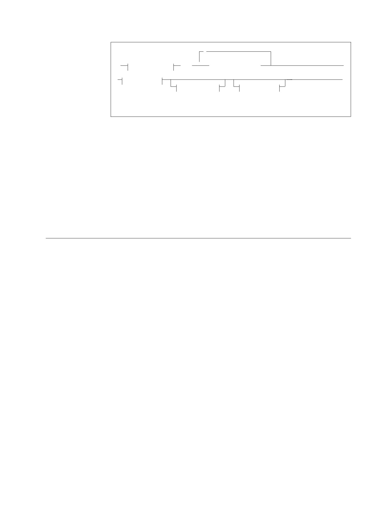
select-clause

INTO

host_variable_list

►

from-clause

►◄

where-clause

with-clause

Figure 18. Format of the SELECT INTO statement

For example, the following statement selects the employee number, last name, and

yearly salary from the EMPLOYEE table where the employee number is '000130'. It

places the result in the host variables EMP, NAME, and PAY:

SELECT EMPNO, LASTNAME, SALARY

INTO :EMP, :NAME, :PAY

FROM EMPLOYEE

WHERE EMPNO = ’000130’

If the number of expressions in the select-list is greater than the number of output

host variables in the INTO clause, a warning flag (called SQLWARN3) in the

SQLCA is set to W. Also, if more than one row satisfies the search condition in a

SELECT INTO statement, an error condition occurs, and the values of the host

variables are unpredictable.

Constructing Search Conditions

One of the most common operations in SQL is to search through a table, choosing

certain rows for processing. A search condition is the criterion for choosing rows.

In the following select-statement example, CODE = 'A' AND PART='B' AND

TYPE='X' constitute the search condition:

SELECT * FROM T1

WHERE CODE = 'A' AND PART='B' AND TYPE='X'

When you are constructing search conditions, be careful to perform arithmetical

operations only on numeric data types, and to make comparisons only among

compatible data types. Graphic data types are compatible only with other graphic

data types. If you use a host variable in an expression, its host language data type

must be compatible with the rest of the expression.

Performing Arithmetic Operations

Whenever an arithmetic or comparison operator has operands of two different

types, the database manager evaluates it in the greater of the two types: FLOAT

takes precedence over DECIMAL, which takes precedence over INTEGER, which

takes precedence over SMALLINT. For example, if the PRICE column is of type

INTEGER and has the value 25, the expression PRICE*.5 will evaluate to 12.5, a

decimal value. The predicate PRICE*.5=12 is false, because the decimal value forces

the predicate to be evaluated in decimal. (Decimal values are stored in

System/390^™ packed decimal format.)

The system computes all floating-point values in normalized form, as described in

the ESA/390 Principles of Operation manual. When a floating-point value is stored in

a table, it may not be stored exactly as entered. For example, an SQL INSERT

Chapter 3. Coding the Body of a Program

statement could specifically insert the constant 3E0 into a column. Internally,

however, the value might actually be stored as 2.9999. Floating-point values may

become even more imprecise when arithmetic operations are performed on them.

You should use the BETWEEN predicate (described later) when comparing

floating-point values.

If the operands of an arithmetic or comparison operator are both single-precision

and double-precision floating-point data, the former is converted to the latter

before any comparison is made or any arithmetic operation performed. If the

equals (=) comparison operator compares these two types of data, the result of the

comparison may not be what you expected. In the following examples, column C1

is defined to contain single-precision floating-point data and column C2 is defined

to contain double-precision floating-point data:

INSERT INTO T1 (C1, C2) VALUES (10.95, 10.95)

SELECT * FROM T1

WHERE C1 = 10.95

SELECT * FROM T1

WHERE C2 = 10.95

SELECT * FROM T1

WHERE C1 = C2

The first and second select statements here will return rows that contain the value

10.95. The third select will not return any rows. This is because the 10.95 cannot be

exactly expressed as a floating-point value. The double-precision floating-point

representation has more significant bits than the single-precision floating-point

representation. When the single-precision floating-point value is converted to

double-precision float, X’00’s are added to the last four bytes of the

double-precision equivalent. The single-precision float data is therefore not equal to

the double-precision float data and hence the search condition in the last select

above is not satisfied.

Decimal numbers have a maximum precision of up to 31 digits. In contrast, a

double-precision floating point number preserves up to approximately 17 digits. So

when a decimal number with precision greater than 17 is promoted to a

floating-point number, digits are lost. Because floating-point numbers can have a

larger magnitude than decimal numbers, the float data type is higher than the

decimal in the data type promotion scheme. The following example shows how

this can cause unexpected results:

SELECT * FROM DEPARTMENT WHERE 1E0 + 12345678901234567890.1

= 12345678901234567890.1;

You would expect this statement to return no rows, because adding one to a

constant makes it unequal to itself. To execute this statement, the system promotes

the two decimal numbers to floating-point values. When this is done, all but the

first 17 digits are lost. When ’1E0’ is added to the first decimal number, > it is not

large enough to change the converted decimal value. The end result is that both

sides of the expression evaluate as being equal. It is therefore important to be

careful when combining floating-point and decimal data types in expressions.

Arithmetic operations between two items of type SMALLINT produce a result of

type INTEGER, in order to avoid possible overflow problems (as might easily

occur in multiplication). When INTEGER or SMALLINT values are used in a

division computation, the result is of type INTEGER, and any remainder is

dropped. (See “Converting Data” on page 48 for conversion information.)

Application Programming

Using Null Values

The system allows nulls in values in a table. A null is a nonexistent value; that is,

it represents a value that is undefined. You can think of a null value as an empty

space, or as a space reserved for later insertion of data.

When null values occur within expressions, the value of the expression is also null.

For example, in the following predicate both SALARY and COMM may be a null

value:

SALARY + COMM < 100

expression1

expression2

If either SALARY or COMM is null, expression1 above is null.

Using the Predicates of a Search Condition

A search condition is a collection of one or more predicates. Each predicate specifies

a test that is applied to the rows of the table. You can connect predicates with the

logical operators AND and OR. For example:

predicate1

AND predicate2

OR predicate3

The keyword NOT can be used to negate a predicate:

predicate1 AND NOT predicate2

The precedence rule among the keywords is as follows:

1. NOT is applied

2. AND is applied

3. OR is applied.

Use parentheses to override this precedence rule if necessary. For example, the

search condition in Figure 19 contains three predicates; it is used to find the rows

of the EMPLOYEE table pertaining to an employee from department D11 who also

has 17 or 18 years of education.

Chapter 3. Coding the Body of a Program

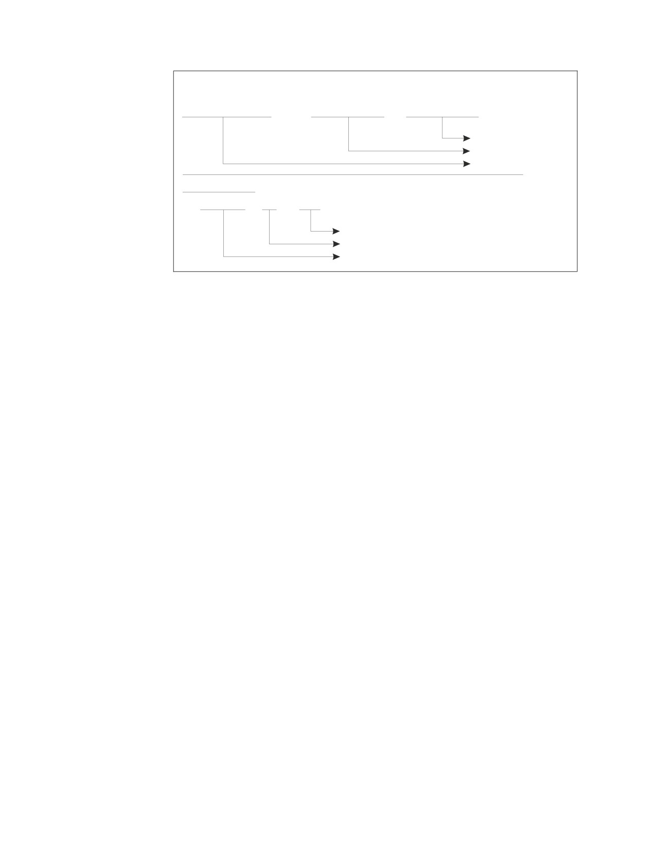
Search Condition:

WORKDEPT='D11'

AND

(EDLEVEL = 17

OR EDLEVEL = 18)

Predicate 3

Predicate 2

Predicate 1

Predicate 1:

WORKDEPT

'D11'

expression

comparison operator

expression

Figure 19. Breakdown of Search Conditions and Predicates

Figure 19 also shows that the format of a predicate is a comparison between two

values or expressions. This format is represented as follows:

expression comparison-operator expression

A comparison-operator may be any of the following:

"equal to"

¬=

"not equal to"

"greater than"

"greater than or equal to"

"less than"

"less than or equal to"

The above symbols are the only comparison operators that you can use in SQL

statements. For example, the system does not recognize ≠ even if it is supported in

the host language. The correct representation of inequality is ¬= or <>.

For a detailed description of search conditions, see the DB2 Server for VSE & VM

SQL Reference manual.

Evaluating Predicates

The following rules apply when the system evaluates predicates:

1. When two character strings are compared, EBCDIC alphabetic ordering is used.

For example:

’A’ < ’B’

’A’ < ’ABLE’

’Z’ < ’35’

’A1’ < ’B’

’a’ < ’A’

2. When two short strings are compared, trailing blanks are not significant. For

example, if the NAME column of a table is of type CHAR(10), you can write

NAME='SMITH' in your search condition, and the condition will be satisfied by

the database value:

'SMITH

Trailing blanks are significant in the LIKE predicate; see the DB2 Server for VSE

& VM SQL Reference manual.

3. In performing an arithmetic operation, if either of the operands is null, the

result of the operation is null.

Application Programming

4. In performing a comparison operation, if either of the expressions is null, the

result of the comparison is unknown, and the row being evaluated does not

qualify for inclusion in the result table.

5. No predicates are permitted on long host variables. Except for LIKE, predicates

are not permitted on long columns.

6. When decimal numbers of different scales are compared, the shorter scale is

extended with trailing zeros sufficient to match the scale of the larger number.

For example, 25.45 is equal to 25.4500.

7. When two graphic strings are compared, the value of the respective data

columns is compared in a manner similar to that used for character data types.

The single character sequencing is generally of no value for graphic ordering.

However, you can specify the sorting sequence of graphic characters in a

graphic column by associating the column with a field procedure. For more

information on field procedures refer to “Using Field Procedures” on page 281.

8. If a query is executed against an empty table, the database manager may not,

for performance reasons, carry out all validation checks. For example, an

invalid date string in a host variable is not flagged as an error unless a row is

being evaluated.

Using Additional Types of Predicates

In addition to the basic predicates that compare two expressions, the system

provides the predicates listed below, which you can use either alone or with other

predicates by including the keywords AND, OR, and NOT to form a search

condition. For detailed information on the rules and use of these predicates, see the

DB2 Server for VSE & VM SQL Reference manual.

v BETWEEN

v IN

v LIKE

v NULL

v EXISTS

v Quantified (SOME, ALL).

Using Functions

There are two types of functions. Column functions apply the function to a group of

values in a column and produce one result value. Scalar functions apply the

function to one or more values in each row and produce a result value for each

row.

Using Column Functions

The column functions are:

AVG MAX MIN SUM COUNT

The argument of a column function is an expression containing a column name

(optionally preceded by DISTINCT or ALL— ALL is the default). The argument

follows the function and must be enclosed in parentheses.

DISTINCT indicates that duplicate values are to be eliminated before the function

is applied. The following example counts the number of different projects that

satisfy the search condition:

SELECT COUNT(DISTINCT PROJNO)

For a detailed discussion of each of the column functions, see the DB2 Server for

VSE & VM SQL Reference manual.

Chapter 3. Coding the Body of a Program

Using Scalar Functions

The scalar functions are:

CHAR

FLOAT

MINUTE

TIMESTAMP

DATE

HEX

MONTH

TRANSLATE

DAY

HOUR

SECOND

VALUE

DAYS

INTEGER

STRIP

VARGRAPHIC

DECIMAL

LENGTH

SUBSTR

YEAR

DIGITS

MICROSECOND

TIME

You can use scalar functions wherever an expression can be used. The first or only

argument of each scalar function is an expression. If the value of any expression is

a null value, the result will be a null value as well, except for the VALUE function.

For a detailed discussion of each of the scalar functions, see the DB2 Server for VSE

& VM SQL Reference manual.

Using Data Types

Assigning Data Types When the Column Is Created

Each column of every DB2 Server for VSE & VM table is given an SQL data type

when the column is created. Table 6 shows the data types and how they are stored

internally.

Table 6. SQL Data Types

SQL Data Type

How Stored

INTEGER or INT

Stored as a signed 31-bit binary integer

SMALLINT

Stored as a signed 15-bit binary integer

DECIMAL[(p[,s])] or

Stored as a packed decimal number of precision p and scale s. Precision is the total

DEC[(p[,s])] ⁴ , ⁵

number of digits; scale is the number of digits to the right of the decimal point. For

example, 251.66 fits in a DECIMAL(5,2) data area. When precision and scale are

calculated, if the precision is greater than 31, leading zeros will be removed until it is

equal to 31. Trailing zeros are not removed. The default scale is 0 and the default

precision is 5.

FLOAT(n) ¹

Stored as a single-precision (4-byte) floating-point number in short System/390

floating-point format, or as a double-precision (8-byte) floating-point number in long

System/390 floating-point format.

CHARACTER[(n)] or

Stored as a character string of fixed length n, where ≤ 254. The default length is 1.

CHAR[(n)] ³

VARCHAR(n) ² , ³

Stored as a varying-length character string of maximum length n, where n ≤ 32767. If

254 < n ≤ 32767, VARCHAR(n) is considered a long string.

LONG VARCHAR ³

Stored as a varying-length character string of maximum length 32767.

GRAPHIC[(n)]

Stored as a string of double-byte character set (DBCS) characters of fixed length n,

where n ≤ 127. The default length is one DBCS character.

VARGRAPHIC(n) ²

Stored as a varying-length string of DBCS characters of maximum length n, where n ≤

16383. If 127 < n ≤ 16383, VARGRAPHIC(n) is considered a long string.

LONG VARGRAPHIC

Stored as a varying-length string of DBCS characters of maximum length 16383.

DATE

Stored as a string of 4 bytes. Each byte is two packed decimal digits. The first two

bytes are the year, the next is the month, and the last is the day.

TIME

Stored as a string of 3 bytes. Each byte is two packed decimal digits. The first byte is

the hour, the next is the minute, and the last is the second.

Application Programming

Table 6. SQL Data Types (continued)

SQL Data Type

How Stored

TIMESTAMP

Stored as a string of 10 bytes. Each byte is two packed decimal digits. The first 4

bytes are the date, the next 3 are the time, and the last 3 are the microsecond.

Notes:

The FLOAT data type refers to either single-precision floating-point data (4

bytes) or double-precision floating point-data (8 bytes).

v REAL and FLOAT(n), where n is from 1 to 21, are synonyms. They are both

stored as 4 bytes.

v FLOAT, DOUBLE PRECISION, and FLOAT(n), where n is from 22 to 53, are

synonyms. They are all stored as 8 bytes.

v When single- and double-precision floating-point data are compared to one

another, the result of the comparison may not be what you expected. See

“Constructing Search Conditions” on page 39.

These data types have some special considerations to watch out for.

v For the CREATE TABLE and ALTER TABLE statements, when VARCHAR(n)

or VARGRAPHIC(n) has “n” greater than 254 or 127 respectively, the

database manager treats the column as a long string when storing and

retrieving data. Long strings are discussed in the next section.

The column is treated as VARCHAR or VARGRAPHIC, however, in two

respects:

- The value stored in the LENGTH and SYSLENGTH columns of

SYSTEM.SYSCOLUMNS is “n”.

- The value returned to the user in the SQLLEN field of the SQLDA is “n”.

When n is less than 255 (VARCHAR) or 128 (VARGRAPHIC) on these

statements, the treatment of the column is unchanged.

v Trailing blanks are not considered relevant in comparisons of VARCHAR or

VARGRAPHIC values, unless these values are either concatenated, returned

to the application program, or used in a scalar function.

For example, if string X1 = "STRING " and string X2 = "STRING" and X3 =

X1 CONCAT X2 then X3 will be equal to "STRING STRING". However, X1 is

considered equal to X2 in a compare statement such as a SELECT...WHERE.

Columns defined with these data types can contain MIXED or BIT data.

NUMERIC is a synonym for DECIMAL, and may be used when creating or

altering tables. In such cases, however, the CREATE or ALTER function will

establish the column (or columns) as DECIMAL.

C application programs can use the decimal data type so that host variables can

match table definitions and do not have to do C numeric conversions for table

columns that are defined as decimal.

Using Long Strings

Defining Long Strings

A long string column is either a LONG VARCHAR, LONG VARGRAPHIC,

VARCHAR(n) (where 254 < n ≤ 32 767), or VARGRAPHIC(n) (where 127 < n ≤ 16

383). Long strings are intended for storage of unstructured data such as text

strings, images, and drawings. For a list of restrictions on the use of long strings,

refer to the section on data types in the DB2 Server for VSE & VM SQL Reference

manual.

Chapter 3. Coding the Body of a Program

Performing Operations on Long Strings

The only operations permitted on long strings are:

v SELECT in an outer-level query (not in a subquery).

v INSERT into the database from an input host variable (not from a constant or

from a subquery). You can, however, insert null values into long strings with the

usual INSERT statement mechanisms. (That is, you are not restricted to host

variables when inserting nulls.)

v UPDATE from an input host variable or UPDATE to the null value. (SET

LONGFIELD=:X and SET LONGFIELD=NULL are permitted, but SET

LONGFIELD=’HELLO’ and SET LONGFIELD=OTHERFIELD are not permitted.)

v DELETE of rows containing long strings.

Programming Tip

The restrictions on the use of long strings can usually be avoided by the

appropriate use of the SUBSTR function.

Using Datetime Data Types

Datetime is a collective DB2 Server for VSE & VM term that includes date, time,

and timestamp. Although datetime values can be used in certain arithmetic

operations and are compatible with certain strings, they are neither strings nor

numbers. Conversely, strings and numbers are not datetime values. A datetime

value is either:

v A DATE, TIME, or TIMESTAMP column value

v A value returned by the DATE, TIME, or TIMESTAMP scalar functions

v A value returned by the CURRENT DATE, CURRENT TIME, or CURRENT

TIMESTAMP special registers.

Datetime values of the same type can be subtracted. If date1 and date2 are DATE

columns, date1 - date2 is a valid expression. Date1 - '01/01/2000' is also a valid

expression because '01/01/2000' is a valid string representation of a date. However,

'01/01/2000' - '12/20/1999' is not valid because strings cannot be subtracted and a

string is interpreted as a date only if the other operand is a value of data type

DATE. Scalar functions are provided to explicitly convert strings to datetime

values. The following expression is valid: DATE('01/01/2000') - '12/20/1999'.

For detailed information on the components and valid formats and lengths of the

date, time, and timestamp data types and the assignment of these data types to

host variables or CHAR-type columns, see the DB2 Server for VSE & VM SQL

Reference manual.

Using Character Subtypes and CCSIDs

Character subtypes and coded character set identifiers (CCSIDs) provide a means

of identifying the character data representation scheme to be used for character

and graphic data in your system. For example, by using a certain CCSID, you can

specify that all character data in your system is single-byte EBCDIC data.

Subtypes are a way of specifying that you want to use the application server

system default CCSID associated with that subtype. CCSIDs apply to both

character and graphic data, while subtypes apply only to character data.

For a detailed description of coded character sets and CCSIDs, see the DB2 Server

for VSE & VM SQL Reference manual.

Application Programming

For most applications, you do not need to specify subtypes or CCSIDs, because the

system defaults can usually meet your character data representation requirements.

If this is not the case, you may have to become familiar with Character Data

Representation Architecture (CDRA). Refer to the section about data integrity

concerns in the Character Data Representation Architecture Reference and Registry

manual for a discussion of using CDRA to meet your requirements.

The following are examples of problems that can be solved by the specification of

CCSIDs or subtypes. The solutions to these problems are discussed in “Assigning

Subtypes and CCSIDs When a Column Is Created” on page 48 and “Assigning

Subtypes and CCSIDs to Data in a Program” on page 48.

v A column is required in a table to contain mixed data (that is, data that can

contain both double-byte and single-byte characters), but the system default

specifies that all newly created columns will be used to contain single-byte

character set data only.

v A table creation program is required that is to be used at multiple sites, all of

which can use different system default subtype and CCSID values. The tables to

be created must have the ability to store data of a particular CCSID.

v An application program written in assembler language must insert data into a

graphic column, but variables with a graphic data type are not supported.

Determining Default Subtypes and CCSIDs

Refer to the SYSTEM.SYSOPTIONS catalog table to determine the application

server system defaults. The rows containing the following values in the

SQLOPTION column are important: CHARSUB, CCSIDSBCS, CCSIDMIXED,

CCSIDGRAPHIC, and CHARNAME.

DB2 Server for VM

For the application requester system defaults, invoke the SQLINIT EXEC

using the QUERY option. The fields that contain important information are

CCSIDSBCS, CCSIDMIXED, CCSIDGRAPHIC, and CHARNAME. (For a

discussion of the SQLINIT EXEC, refer to the DB2 Server for VSE & VM

Database Administration manual.)

Examples of items that assume application requester system defaults are input and

output SQLDA elements (the default can be overridden), and host variables.

The following are examples of items that assume application server system

defaults:

v Columns (default can be overridden)

v Special registers.

The following are examples of items that assume application requester system

defaults:

v Input and output SQLDA elements (default can be overridden)

v Host variables.

For information on setting system defaults, refer to the DB2 Server for VM System

Administration or the DB2 Server for VSE System Administration manual.

Chapter 3. Coding the Body of a Program

Assigning Subtypes and CCSIDs When a Column Is Created

There are three ways to assign subtypes or CCSIDs to a column:

v Use the application server system defaults.

v Use the preprocessor parameters CHARSUB, CCSIDSBCS, CCSIDMIXED, and

CCSIDGRAPHIC to override the system default for columns created by the

CREATE TABLE and ALTER TABLE statements in the package. (See

“Preprocessing the Program” on page 114 (DB2 Server for VM) “Preprocessing

the Program” on page 156 (DB2 Server for VSE) for information on these

parameters.)

v Use the subtype or CCSID clause in a column’s definition within the CREATE

TABLE or ALTER TABLE statement to override the application server system

default or the preprocessor default. (For more information on these statements,

refer to the DB2 Server for VSE & VM SQL Reference manual.)

Assigning Subtypes and CCSIDs to Data in a Program

There are two ways to assign subtypes or CCSIDs to the data items in a program:

v Use application requester system defaults

v Execute the SQL statement using dynamic SQL so that the data items can be

described in a user-defined SQLDA. A CCSID can be assigned to each data item

in the SQLDA.

For examples of how to build an SQLDA that contains CCSID information, see

Chapter 7, “Using Dynamic Statements,” on page 215. For a more detailed

discussion on using the SQLDA, refer to the DB2 Server for VSE & VM SQL

Reference manual.

Converting Data

For the database manager, the operands in an assignment or comparison operation

must be compatible. For example, a character string cannot be compared to a

numeric string, a graphic string cannot be compared to a character string, and an

arithmetic operation cannot contain a character string operand. Refer to the DB2

Server for VSE & VM SQL Reference manual for more details about compatible data

types.

Operands that are compatible but are not identical in data types, lengths, datetime

formats, or CCSIDs, can be used in assignment and comparison operations but

require data conversion as follows:

v For assignment operations, conversion is done before the data is assigned. For

example, if a host variable is defined as a SMALLINT field and a column is

defined as INTEGER, a SELECT INTO operation converts the INTEGER column

to SMALLINT before it is assigned to the host variable. In this situation,

overflow may occur if the value is too large to fit into a SMALLINT field.

Depending on the data types and the host language, some data may be lost. The

DB2 Server for VSE & VM SQL Reference manual discusses potential data loss in

the assignment of COBOL integers.

To retrieve a datetime value, (that is, a DATE, TIME, or TIMESTAMP), it must

be assigned to a character string host variable. The assignment operation

converts the datetime value to a character string representation. Whenever a

string representation of a datetime value is used in any other operation with a

datetime value, the operation is performed with a temporary copy of the string

that has been converted to the data type of the datetime value.

Application Programming

If a conversion error occurs when the database manager assigns a value to a

host variable in the INTO clause of a SELECT or FETCH statement, and if you

have provided an indicator variable for the affected host variable, the system

returns the following:

- A value of −2 in the indicator variable

- An undefined value in the host variable

- Warning values in both SQLCODE and SQLSTATE that are appropriate for

the condition.

If you have not provided an indicator variable, both SQLCODE and SQLSTATE

return error codes (a negative value for SQLCODE, and a data exception for

SQLSTATE).

v For comparison operations, one field may be converted if necessary to match the

data type, length, or CCSID of another. For example, if two character strings in a

comparison operation have different CCSIDs (one is an SBCS string and the

other is a mixed string), a temporary copy of the SBCS data is converted to the

mixed data CCSID before the data is compared.

For more information about data conversion and conversion errors, see the

discussion about assignments and comparisons in the DB2 Server for VSE & VM

SQL Reference manual.

Summarizing Data Conversion

Data conversion is summarized in tabular form in the DB2 Server for VSE & VM

SQL Reference manual. Overflow (loss on the left) or truncation (loss on the right)

may occur on some conversion attempts.

Truncating Data

Truncations are handled differently for numeric, character, and datetime data.

Numeric data

Truncation of zeros on the left, or of the fractional

part of decimal or floating-point values

(single-precision or double-precision) takes place

without error or warning. Any other loss of data

on conversion is an overflow error. If overflow

occurs in an outer select and an indicator variable

is supplied for the host variable, the indicator

variable is set to −2 and a positive SQLCODE is

returned; otherwise, a negative SQLCODE is

returned.

Character data

When output from the database manager does not

fit into a host variable, a warning is returned.

SQLWARN1 is set to indicate truncation. In this

case, if you provide an indicator variable, the value

within it denotes the actual length of the variable

in characters before truncation.

When an input character string value does not fit

into a DB2 Server for VSE & VM column, an error

results.

Whenever truncation occurs, it follows specific

rules depending on the character subtype involved.

Also, padding may occur when a string is assigned

to either a fixed-length host variable or to a

fixed-length column and the source string is

Chapter 3. Coding the Body of a Program

shorter than the length of the target. Padding, like

truncation, follows rules depending on subtype.

These rules are in the DB2 Server for VSE & VM

SQL Reference manual.

SBCS and mixed are the only two types of

character data truncation. In mixed truncation, the

integrity of target data is ensured. For example, if

’ab<▌CCDDEE▐>cd’ is truncated to a length of 6, the

result with mixed truncation is ’ab<▌CC▐>’. The

system counts to byte 6. Because this would split a

double-byte character, the number of bytes is

rounded to the next lowest whole number. It also

always ensures that the < and > characters

correctly identify the double-byte characters.

Table 7 shows the type of truncation that occurs

depending on the subtype of the source and target

data.

Table 7. Truncation Types

Subtype of Source

Subtype of Target

Result

Mixed

Mixed truncation

SBCS

SBCS truncation

Mixed

SBCS

SBCS truncation¹

SBCS

Mixed

SBCS truncation¹

Note:

1. If the source data contains DBCS data, a conversion error occurs during SBCS

truncation.

Table 8 shows the results of SBCS and mixed

truncation when selecting ’ab<▌CCDDEE▐>fg’ into

various host variables:

Table 8. Examples of Mixed Data Truncation and SBCS Truncation

Target Host Variable

SBCS Truncation

Mixed Truncation

CHAR(6)

’ab<CCD’

’ab<▌CC▐>’

CHAR(7)

’ab<CCDD’

’ab<▌CC▐>’

VARCHAR(7)

’ab<CCDD’

’ab<▌CC▐>’

Note: For mixed data, the only difference between

the second and the third example is the

length of the resulting VARCHAR string. A

blank is added to the fixed string.

TIME data

When the seconds part of a retrieved ISO, JIS, or

EUR format TIME value is truncated, SQLWARN1

is set to indicate that truncation has occurred. The

seconds that are truncated are placed in the

indicator variable if one is provided.

TIMESTAMP data

On output, any portion of the microseconds part of

a TIMESTAMP may be truncated (including the

decimal point). However, no warning is given

Application Programming

(SQLWARN1 is not set). If an indicator variable is

provided, it is unchanged.

For more information about how computations are performed internally or how

overflows can occur, refer to the section about arithmetic operations in the DB2

Server for VSE & VM Database Administration manual.

Using a Double-Byte Character Set (DBCS)

DBCS characters can be used in identifiers, constants, and data in DB2 Server for

VSE & VM programs. Strings containing DBCS characters are formatted as

<▌XXXX▐>, where < represents the shift-out character, and > represents the shift-in

character. Each XX represents one double-byte character set character. The <>

delimiters are single-byte character set (SBCS) characters.

In identifiers, characters constants, and character data, the delimiters are significant

so redundant delimiter pairs are not removed. For example, the following strings

of DBCS characters are not equivalent:

<▌AABB▐><▌CCDD▐> and <▌AABBCCDD▐>

In graphic data and constants, the delimiters are not significant.

Each DBCS character requires 2 bytes for its representation; therefore, an even

number of bytes must be between the < and >. The number of bytes used to

represent a string of DBCS characters is equal to:

2 * the number of DBCS characters + 2 (for mixed data)

2 * the number of DBCS characters (for graphic data)

Strings of DBCS characters cannot span lines, whereas mixed strings containing

strings of DBCS and SBCS characters can span lines if each string of DBCS

characters in the mixed string is on one input record. For a discussion of the rules

for using DBCS characters in constants, see “Using Character Constants” on page

57 and “Using Graphic Constants” on page 58.

To use DBCS characters in application programs, you must know the following:

v To use host identifiers that contain DBCS characters in DB2 Server for VM, your

compiler must support DBCS and the application requester must have the DBCS

option set to YES. To check whether this setting is correct, do an SQLINITQRY; if

you need to change this setting, issue an SQLINIT with the DBCS option set to

YES. (For a detailed discussion of the SQLINIT EXEC, see the DB2 Server for VSE

& VM Database Administration manual.)

v To use host identifiers in DB2 Server for VSE, the DBCS option in the

SYSTEM.SYSOPTIONS catalog must be set to yes. Your compiler must also

support DBCS.

v To use SQL identifiers that contain DBCS characters, the application server must

support DBCS characters and mixed data. To verify this for the application

server, make sure that in the SYSTEM.SYSOPTIONS catalog table the

CHARNAME setting identifies a mixed character set and the DBCS setting is

YES. In addition, DBCS characters must be permitted in the particular identifier.

For a discussion of rules for using DBCS characters in identifiers, refer to the

DB2 Server for VSE & VM SQL Reference manual.

v To use host variables with graphic data type, the preprocessor must allow a

graphic data type for the host language of the source program. This is true for

COBOL and PL/I only in DB2 Server for VSE. The DB2 Server for VM

Chapter 3. Coding the Body of a Program

preprocessors that allow graphic data type are COBOL and PL/I. If you need

this facility when using another language, see the appendix for that language for

a discussion of alternative actions.

v To use graphic and mixed constants (that is, character constants that contain

DBCS characters) in an application program, the DB2 Server for VM application

server and application requester or DB2 Server for VSE application server must

support mixed data. To verify this for the application server, make sure that the

CHARNAME setting in the SYSTEM.SYSOPTIONS catalog table identifies a

mixed character set. To verify this for the DB2 Server for VM application

requester, issue an SQLINIT command with the QRY option. The CHARNAME

value returned identifies a mixed character set. For a discussion of character sets,

refer to > the DB2 Server for VM System Administration or the DB2 Server for VSE

System Administration manual. If the DB2 Server for VM application requester

does not support DBCS characters, you can obtain this support by using the

SQLPREP GRaphic option (available to COBOL and PL/I only).

Using Expressions

An expression refers to a column, a constant, a host variable, an SQL special register

(for example, the USER special register), the SQL keyword NULL, a column

function, a scalar function, an arithmetic expression, or any of these that can be

connected by the concatenation operator. (The concatenation operator is discussed

later in this chapter.) Using expressions, you can do calculations on data as part of

a query. The calculations are performed before the data is returned to your

program.

Table 9 shows a simple arithmetic expression:

Table 9. Breakdown of an Arithmetic Expression

Expression

(BONUS

:MARKDOWN * .80)

constant

host variable

column name

Using Arithmetic Operators

There are four arithmetic operators that you can use:

multiplication

division

addition

subtraction

Usually, the system reads an arithmetic expression from left to right, first applying

any negations, then any multiplication or division operations, and then finally any

additions and subtractions. For example, in the following expression:

BONUS - :MARKDOWN * .80

The system would take the value of the host variable MARKDOWN, multiply it by

.80, and then subtract the result from the bonus.

You can change this order-of-precedence by using parentheses. For instance, if the

above example were coded:

(BONUS - :MARKDOWN) * .80

Application Programming

The system would first subtract MARKDOWN from BONUS, and then multiply

the result by .80. The two results would probably end up being quite different.

Host variables can be used in arithmetic expressions. For example:

PRICE * :QUANTITY + 1.44

As mentioned earlier, you must precede the names of host variables by a colon (:)

to distinguish them from column names. That is, the following is interpreted as a

host variable:

:PROJNO

The following, however, is interpreted as a column name:

PROJNO

Numeric constants can stand alone or be used in arithmetic combination with other

constants or host variables or column names to form expressions. All three of the

following are valid expressions:

200

-798.9768

PRICE * :QUANTITY + 1.44

Character constants cannot be used in arithmetic combinations, except when a

character string representing a datetime value is used in datetime arithmetic. The

following expression is valid:

HIRE_DATE - ’2000-01-01’

The following expression is not valid:

’FUDGE’*’GUMDROP’+’LEMON’

If you attempt to combine two pieces of data that do not have compatible data

types with arithmetic operators, an error code is returned. The system performs

data conversion on different types of data that are compatible.

Using Special Registers

Any of the following special registers can be used wherever an expression of the

appropriate data type is used:

v CURRENT DATE (defined as DATE)

v CURRENT SERVER (defined as CHAR(18))

v CURRENT TIME (defined as TIME)

v CURRENT TIMESTAMP (defined as TIMESTAMP)

v CURRENT TIMEZONE (defined as DECIMAL(6,0))

v USER (defined as CHAR(8))

Using CURRENT DATE, TIME, and TIMESTAMP: The values of all datetime

special registers in the same statement are based on the same time-of-day (TOD)

clock reading.

In the examples below, one uses the select-statement and the other uses the

UPDATE statement.

SELECT CURRENT DATE, PRSTDATE

FROM PROJECT

ORDER BY PRSTDATE

UPDATE PROJECT SET PRSTDATE = CURRENT DATE,

PRENDATE = ’2000-01-20’

WHERE PROJNAME = ’OPERATION’

Chapter 3. Coding the Body of a Program

Using CURRENT TIMEZONE: The CURRENT TIMEZONE is a signed

time-duration containing the local time zone value. A negative value represents

differentials west of the Greenwich-Mean-Time (GMT). A positive value represents

differentials east of the GMT. CURRENT TIMEZONE can be used to convert local

time into GMT by subtracting CURRENT TIMEZONE from local time. CURRENT

TIMEZONE can be subtracted from a TIME or TIMESTAMP data type.

The following example shows a query that involves CURRENT TIMEZONE.

SELECT RECEIVED - CURRENT TIMEZONE

FROM IN_TRAY

Using CURRENT SERVER: This special register holds the server name of the

application server currently connected. It has a CHAR(18) data type.

The following example shows a query that includes the CURRENT SERVER special

SELECT ID, INDATE, INTIME

FROM SAMP1

WHERE INRDB=CURRENT SERVER

Using USER: This special register is evaluated as the currently connected userid

that is, the user ID of the person who is running the program, regardless of who

preprocessed it. USER behaves exactly like a fixed-length character string constant

of length 8, with trailing blanks if the user ID has fewer than eight characters.

Notes:

1. You cannot use this keyword in an arithmetic expression (for example,

USER+3).

2. You can use it in a predicate where you compare it to a character string (for

example, USER = 'JIM').

3. You can use it in the LIKE predicate, where it is treated as a pattern.

4. You can, with some restrictions, use it in the SET clause of an UPDATE

statement, or in the VALUES clause of an INSERT statement. In both cases, the

data in the target column must be character data type (CHAR or VARCHAR).

The following is a valid expression that includes the USER special register:

SELECT *

FROM SYSTEM.SYSCATALOG

WHERE CREATOR = USER

Concatenating Character and Graphic Strings

You can use the concatenation operator (CONCAT) to concatenate character strings

or graphic strings. Long strings cannot be used with the concatenation operator.

The following example shows the concatenation of employees’ last names and jobs,

separated by a hyphen:

SELECT LASTNAME CONCAT '-' CONCAT JOB FROM EMPLOYEE

For a full description of this operation, including rules for character subtypes and

CCSIDs, see the DB2 Server for VSE & VM SQL Reference manual.

Note: The || symbol is a synonym for CONCAT. Because the | symbol is not in a

consistent position in all code pages, the use of || could impair code

portability.

Application Programming

Using Host Variables

As previously stated, host variables are host program variables that are declared in

an SQL declare section. The host program can use these variables to interact with

the database manager.

You can use host variables to pass data to or receive data from the database

manager. Host variables used to contain column data or data used to evaluate an

expression are called main variables. The data type and length attributes of a main

variable depend on the data type and length of the column or expression to which

the variable relates.

You can also use host variables to communicate information to and from the

database manager about the contents of the main variable. If a host variable is

used in this context, it is an indicator variable. Only use host variables that are

declared with a data type equivalent to 15-bit integer as indicator variables. Refer

to “Using Indicator Variables” on page 59 for a description of their use.

Several SQL statements permit the use of host variables. Refer to the DB2 Server for

VSE & VM SQL Reference manual for the syntax of these SQL statements. The

syntax diagrams indicate whether host variables are permitted or required.

For a description of how to declare host variables, refer to the appropriate host

language appendix.

Using Host Structures

A host structure is a special form of host variable. It is any two-level structure or

substructure declared in an SQL declare section. Host structures can replace all or

part of a host_variable_list. A host_variable_list can contain references to more than

one host structure.

The elements of the host structure comprise the list of main variables in the

host_variable_list. To provide indicator variable support for the elements of the host

structure, you must use an indicator array. An indicator array of n elements

provides indicator variable support for the first n elements of the host structure.

The elements of host structures and structures that contain host structures can

replace scalar host variables in an SQL statement. You can qualify the element

name with the names of parent structures and substructures. The following syntax

diagram shows the format of a structure element reference.

►►

element_name

►◄

struct_name.

It is only necessary to qualify a structure or element name where failure to do so

would result in an ambiguous reference.

Elements of indicator arrays cannot be used as host variables and host structures

(or structures that contain host structures) cannot be declared as arrays or contain

arrays.

Chapter 3. Coding the Body of a Program

Refer to the appropriate host language appendix for rules on the declaration of

host structures and indicator arrays. Refer to the DB2 Server for VSE & VM SQL

Reference manual for more information on the use of host structures and indicator

arrays in SQL statements.

Using Constants

Constants (also called literals) can be numeric or character data. They are fixed

values that can be coded into SQL statements. Like host variables, they are used in

various clauses in a number of different SQL statements.

The following example shows a character string constant coded in a WHERE

clause:

DECLARE C CURSOR FOR

SELECT *

FROM EMPLOYEE

WHERE LASTNAME = ’PEREZ’

Constants can be used in the SELECT clause to set up a new column in the result

table, which has the specified constant in each of its occurrences. For example, the

statement:

DECLARE C CURSOR FOR

SELECT LASTNAME, ’WOW’, 100.0

FROM EMPLOYEE

WHERE COMM > 3200

would have the following result table:

LASTNAME

EXPRESSION 1

EXPRESSION 2

___________

_______________

_________________

LUCCHESI

WOW

100.0

HAAS

WOW

100.0

THOMPSON

WOW

100.0

GEYER

WOW

100.0

Using Numeric Constants

Integer constants consist of a number with an optional sign, such as -56, 103, or

+786. (If you do not include a sign, the system assumes that the number is

positive.) All integer constants are 4 bytes long; that is, there are no constants with

a data type of SMALLINT.

Decimal constants consist of a number with a decimal point, such as 78.9687,

-.00132, 64570., or +1672.80. If you do not supply a decimal point, the constant is

interpreted as an integer. In storage, the number occupies a maximum of 16 bytes.

Precision p, where 1 ≤ p ≤31, is the total number of digits. Scale s, where 0 ≤ s ≤p,

is the number of those digits that are to the right of the decimal point. Leading

and trailing zeros are included in both precision and scale. When the precision and

scale are calculated, if the precision is greater than 31, leading zeros are removed

until the precision is equal to 31. Trailing zeros are never removed. When decimal

data values are multiplied or divided, an overflow condition may occur.

Consider the following:

a string of thirty one 9’s. * 1.0

Application Programming

The string of 9’s is treated as DECIMAL(31,0) and 1.0 as DECIMAL(2,1). The

precision and scale of the product will then be 31 and 1 (DECIMAL(31,1)),

respectively. This will result in a decimal overflow and an arithmetic exception will

occur.

This decimal overflow, can be prevented by changing the constant '1.0' to '1.' This

would define this constant as DECIMAL (1,0) and the resulting product as

DECIMAL (31,0) instead of DECIMAL (31,1). If an expression contains decimal

constants, you can influence its precision and scale by adding leading or trailing

zeros to those constants.

A floating-point constant is an integer or a decimal constant followed by an

exponent marked by the letter E. The E must be followed by an exponent. The 1E0

is acceptable and evaluates to 1. All these are permissible floating-point constants:

-2E5, 2.2E-1, .2E6, +5E+2 or 4E0. All floating-point constants are double-precision in

the system.

Using Character Constants

Character string constants are coded within quotation marks, and are

varying-length character strings of letters, digits, or special characters, such as

'SMITH', '52', or 'k@r -5B'. A character constant implicitly assumes either a FOR

SBCS DATA or a FOR MIXED DATA attribute. You cannot assign the FOR BIT

DATA attribute to a character constant. The constant is assumed to have a subtype

of SBCS unless the following conditions are true. If the following conditions are

true, the constant is assigned a subtype of mixed.

v The application server supports mixed data.

v The constant contains mixed data.

Mixed data is composed of a mix of SBCS and DBCS characters in one string. The

DBCS portions of the string must be correctly formatted strings of DBCS

characters. (For a discussion of the format and rules for using strings of DBCS

characters, see “Using a Double-Byte Character Set (DBCS)” on page 51.) An

example of mixed data is:

’abc<▌DEFG▐>hi<▌JKLM▐>nop’

where abc, hi, and nop represent SBCS characters, and ▌DEFG▐ and ▌JKLM▐ represent

DBCS characters.

To obtain a single quotation mark in a string of SBCS characters, you must code

two consecutive single quotation marks. For example, the constant ’DON’’T GO’ is

interpreted as DON’T GO. To obtain a single quotation mark in a string of DBCS

characters, you only need to code a single quotation mark. Refer to the DB2 Server

for VSE & VM SQL Reference manual for more information on mixed strings of

SBCS and DBCS characters.

You can also code a character constant using its hexadecimal representation.

Hexadecimal constants are treated like regular character constants. In DB2 Server

for VM, hexadecimal constants are converted from the application requester default

CCSID to the application server default CCSID before they are used.

The hexadecimal representation of a constant value must be enclosed within single

quotation marks and preceded by an X. For example:

X’2D’

X’C1C2C3C4’

X’4256457D’

Each pair of hexadecimal numbers (0-9, A-F) represents a single byte. (Either

uppercase or lowercase letters can be used.) Therefore, the number of hexadecimal

Chapter 3. Coding the Body of a Program

numbers must be even and, when representing a DBCS character in a mixed

constant, it must be a multiple of 4 (each DBCS character occupies 2 bytes in

storage).

You can use hexadecimal constants to represent SBCS and mixed character data

only. The maximum size for hexadecimal constants is 254 hexadecimal digits (that

is, 127 SBCS characters or 63 DBCS characters).

The following is a valid expression using a hexadecimal constant:

LASTNAME CONCAT X’FF’ CONCAT FIRSTNME

Using Graphic Constants

Graphic string constants are fully supported in COBOL and PL/I programs, but

with different formats. The system supports three formats of the graphic constant:

the SQL format and two PL/I formats.

The SQL format of the graphic constant is:

G’<▌XXXX▐>’

Note: N is a synonym for G.

The G identifies the constant that follows as graphic; the <▌XXXX▐> is any valid

string of DBCS characters, and the single quotation marks delimit the constant. You

do not need to double the quotation marks in a graphic constant to obtain a single

quotation mark. Use this format of the graphic constant in all situations except

static SQL statements in PL/I programs.

The PL/I formats of the graphic constant are:

1. ’<▌XXXX▐>’G

2. <▌@’XXXX@’@G▐>

Note: N is a synonym for G.

Again, the G indicates that the constant is a graphic constant, and that the string

bound by < and > must be a valid string of DBCS characters. In the second format,

the single quotation marks and the G are within the string of DBCS characters;

they are the DBCS format of the quotation mark and the G. In the second format,

to obtain a single DBCS quotation mark, double the occurrence of the DBCS

quotation mark within the string of DBCS characters. Use either of these formats of

the graphic constant in static SQL statements in PL/I programs.

The PL/I preprocessor converts PL/I format graphic constants into SQL format

graphic constants (G'<▌XXXX▐>') when they appear in SQL statements. This is done

before passing the SQL statement to the application server for processing.

Therefore, some DB2 Server for VSE & VM messages for incorrect syntax may refer

to the SQL format of the constant, even though a PL/I format constant was coded

in your program.

Graphic constants assume the default graphic CCSID. Subtypes do not apply to

graphic data. For example, you cannot assign the FOR BIT DATA attribute to a

graphic constant. For detailed information on CCSIDs and subtypes, see “Using

Character Subtypes and CCSIDs” on page 46.

Application Programming

For information on the rules for the format and use of strings of DBCS characters

with DB2 Server for VM, see “Using a Double-Byte Character Set (DBCS)” on page

51.

Using Date and Time Constants

A datetime constant is a character string constant or a decimal constant in a

datetime context, as shown in the following examples:

END_DATE - ’1999-09-13’

END_DATE - 10000101.

In the first example, '1999-09-13' is a datetime character string constant; in the

second, 10000101. is a decimal constant. A datetime decimal constant is a date

duration, a time duration, or a timestamp duration. A date duration represents a

number of years, months, and days, and is expressed as a DEC(8,0) number. A

time duration represents a number of hours, minutes, and seconds, and is

expressed as a DEC(6,0) number. A timestamp duration represents a number of

years, months, days, hours, minutes, seconds, and microseconds, and is expressed

as a DEC (20,6) number.

For more detailed information on date and time values, as well as durations, see

“Using Datetime Values with Durations” on page 278.

Using Indicator Variables

Using indicator variables is optional in a host-variable reference. In static SQL

statements, indicator variables can be used to indicate that the corresponding host

variables should be treated as null values or truncated values. Output indicator

variables appear in the INTO clause of a SELECT or FETCH statement, and are

associated with output that is passed from the database to the application

program. Input indicator variables appear in the predicates of WHERE and

HAVING clauses, in the SET clause of an UPDATE statement, with VALUES in an

INSERT statement or in the SELECT clause, and are associated with input that is

passed from the application program to the database.

Output indicator variables should always be used wherever null values are

allowed in the database. Input indicator variables can be used to put null values

into the database. They should, however, not be used in predicates unless there is a

very good reason for doing so, because there may be a significant cost in

performance.

Refer to the DB2 Server for VSE & VM SQL Reference manual for a description of

the format of a host-variable reference that contains an indicator variable.

The following example illustrates the use of indicator variables.

SELECT FIRSTNME, LASTNAME

INTO :FNME:FNMEIND, :LNME

:LNMEIND

FROM EMPLOYEE WHERE WORKDEPT = ’A00’

In this example, the indicator variable FNMEIND provides indicator variable

support for the main variable FNME. The indicator variable LNMEIND provides

indicator variable support for the main variable LNME.

The following notes on the use of indicator variables are grouped according to the

type of indicator variable to which they apply.

Chapter 3. Coding the Body of a Program

Notes Common to Both Input and Output Indicator Variables

1. The indicator variable must be of a host language data type equivalent to an

SQL SMALLINT.

2. A negative indicator variable indicates a null value for its main variable.

Notes on Input Indicator Variables

When using input indicator variables, be aware of the following:

1. Input indicator variables can be used to indicate that a column value is to be

set to null (when the indicator variable is negative). If you provide an input

indicator variable and assign it a negative value, the null value is inserted in

the column value for the row. If the indicator variable is zero or a positive

value, the main variable is inserted. Truncation does not apply to input

variables.

2. A negative indicator variable can be used in static SQL for any of the following

predicates:

v The basic comparison ones (such as = or >)

v BETWEEN

v IN

v LIKE

v The quantified ones (ANY, ALL)

See the DB2 Server for VSE & VM SQL Reference manual for the different sets of

rules for truth values for these predicates.

3. Do not use input indicator variables in search conditions (WHERE or HAVING

clauses) to test for null values. The correct way to test for nulls is with the

NULL predicate (described earlier):

WHERE MGRNO IS NULL

Correct

This will return every row where MGRNO is null.

WHERE MGRNO = :MGR:MGRIND

Incorrect

If MGRIND has been set negative to make MGR null, the truth value is

“UNKNOWN”, and nothing will be returned.

4. On the other hand, there are cases where setting up a negative input indicator

variable in the predicate can prove useful and efficient. For example, if an

application prompts the user to interactively supply information that will

identify an employee (by either number or name), you can design the program

to use only one select-statement to extract the indicated employee data from the

database.

Here is the pseudocode:

get either empno or lastname from user

if empno is entered then empnoind = 0, else empnoind = -1

if lastname is entered then nameind = 0, else nameind = -1

SELECT * FROM EMPLOYEE

WHERE EMPNO = :EMPNO:EMPNOIND

OR LASTNAME = :NAME:NAMEIND

Application Programming

Notes on Output Indicator Variables

When using output indicator variables, be aware of the following:

1. The value returned in an output indicator variable is coded as shown in

Table 10.

2. Output indicator variables are optional. If a null value is returned, however,

and you have not provided an indicator variable, a negative SQLCODE and an

error SQLSTATE are returned to your program. If your data is truncated and

there is no indicator variable, no error condition results. See “Converting Data”

on page 48 for more information about truncation.

Table 10. Values Returned in Output Indicator Variables

Value Returned

Meaning

Denotes that a non-null value that has been returned in the

associated host variable is not null.

Denotes that the value associated with the host variable is null,

and should be treated exactly the same way as null column

values. A -1 denotes that the null value resulted from a normal

operation. A -2 denotes that the null value resulted from either a

conversion error or an error while evaluating an arithmetic

expression in an outer-select clause.

Denotes that the system truncated the returned value in the

associated host variable because the host variable was not of

sufficient length.

In addition, if the truncated item was a DBCS character or a string

of DBCS characters, the indicator variable contains the length in

characters before truncation. If the truncated item was a TIME

value, truncated at its seconds part, the indicator variable contains

the seconds. The SQLWARN1 warning flag in the SQLCA is set to

'W' whenever truncation occurs.

Using Views

Views allow multiple users to see different presentations of the same data. For

example, several users may be operating on a table of data about employees. One

may see data about some employees but not others; another may see data about all

employees but none of their salaries; and a third may see data about employees

joined together with some data from another table. Each of these users is operating

on a view that is derived from the real table of data about employees. Each view

appears to be a table and has a name of its own.

You can create views with authorization statements to control access to sensitive

data. For example, you might create a view based on a GROUP BY query that

gives certain users access to the average salary of employees in each department,

but prevents them from seeing any individual salaries.

A view is a dynamic “window” on tables. When you update a real table, you can

see the updates through a view; when you update a view, the real table underlying

the view is updated. There are, however, restrictions on modifying tables through a

view.

Because a view is not physically stored, you cannot create an index on it. However,

if you create an index on the real table underlying a view, you may improve the

performance of queries on the view.

Chapter 3. Coding the Body of a Program

Creating a View

►► CREATE VIEW view_name

►

(

▼

column_name

)

► AS subselect

►◄

WITH CHECK OPTION

In the following example, a view is created from the EMPLOYEE table:

CREATE VIEW PHONEBOOK (FNAME, LNAME, NUMBER, DEPART, JOBTITLE) AS

SELECT FIRSTNME, LASTNAME, PHONENO, WORKDEPT, JOB

FROM EMPLOYEE WHERE JOB <> ’PRES’ WITH CHECK OPTION

The CREATE VIEW statement causes the indicated select-statement to be stored as

the definition of a new view, and gives a name to the view and (optionally) to each

column in it. If you do not specify the column names, the columns of the view

inherit the names of the columns from which they are derived.

You must specify a name for any view column that is not derived directly from a

single table column (for example, if a view column is defined as AVG(SALARY) or

SALARY+COMMISSION). Columns derived in this manner are often called virtual

columns, (and contain virtual data). You must also specify new column names if the

selected columns of the view do not have unique names (for example, if the view

is a join of two tables, each of which has a column named PROJNO).

In general, the data types of the columns of the view are inherited from the

columns on which they are defined. If a view column is defined on a function, the

data type of the view column will be the data type of the function result. (For

more details on functions, refer to the DB2 Server for VSE & VM SQL Reference

manual.)

If you want to prevent the execution of subsequent inserts or updates to the view

that involve data that is outside the domain of the view’s definition (as specified in

the WHERE clause of its subselect), you can add the WITH CHECK OPTION

clause. This clause, however, is not allowed for updateable views that are built on

subqueries. The checking that is performed at insert or update time is performed

according to a set of rules that cover the situation in which a view is dependent on

other views. See the DB2 Server for VSE & VM SQL Reference manual for these

rules.

Some other considerations when creating views are:

v Internal database manager limitations restrict a view to approximately 140

columns. The number of referenced tables, lengths of column names, and

WHERE clauses all further reduce this number.

v If the subselect in a view definition has a “SELECT *” clause, the view has as

many columns as the underlying table. If columns are later added to the

underlying table by ALTER statements, the new columns will not appear in the

view (unless you drop and re-create the view).

Application Programming

The name of the view must be unique among all the tables, views, and

synonyms that you have already created. You can refer to another user’s views,

if so authorized, by using the owner-name as a prefix (for example,

SMITH.PHONEBOOK).

You can define a view in terms of another view: that is, the subselect that defines

a view may refer to one or more other views. In this case, follow the rules listed

under “Using Views to Manipulate Data” on page 64.

There is no ORDER BY clause in a subselect; therefore, like a table, a view has no

intrinsic order. (Of course, you can specify an ORDER BY clause when you write

queries against the view.)

Host variables are not permitted in a CREATE VIEW statement. (For example,

predicates such as PRICE = :X are not permitted.)

The owner of the view is considered to be the authorization ID under which the

program is preprocessed.

When you define a new view, you receive the same privileges that you have on

the underlying table. If you possess these privileges with the GRANT option,

you can grant privileges on your view to other users. (See Chapter 10,

“Assigning Authority and Privileges,” on page 269 for information on the

GRANT option.) If the view is derived from more than one underlying table,

you receive the SELECT privilege, provided that you have this privilege on all

the tables from which it is derived. (If you have no privileges on the underlying

tables, the CREATE VIEW statement returns an error code.) Only the SELECT

privilege is possible, because multi-table views do not permit insertion, deletion,

or update.

Primary keys and foreign keys (discussed in “Ensuring Data Integrity” on page

289) cannot be defined on a view.

If you defined your view on a table that has a primary key, and you make

changes to that view, the view should contain all the columns of the key.

The subselect is not executed when the view is created, which means that

semantic errors (for example, specifying "WHERE COL = '10'" when COL is a

decimal column) are not detected until the view is used. To determine whether a

statement contains semantic errors, you can enter 'SELECT *' against the view

after creating it.

Querying Tables through a View

You can write queries (select-statements) against views exactly as if they were real

tables. When you make a query against a view, the query is combined with the

definition of the view to produce a new query against real stored tables. This

query is then processed in the usual way. For example, the following query might

be written against the view PHONEBOOK that was defined under “Creating a

View” on page 62:

SELECT FNAME,LNAME

FROM PHONEBOOK

WHERE DEPART = ’D11’

ORDER BY 2

The system combines the query with the definition of PHONEBOOK, and

processes the resulting internal query:

SELECT FIRSTNME, LASTNAME

FROM EMPLOYEE

WHERE JOB <> ’PRES’

AND WORKDEPT = ’D11’

ORDER BY 2

Chapter 3. Coding the Body of a Program

During the processing of a query on a view, the system may detect and report

errors (by a negative SQLCODE) in either of two phases:

v The combination of the query with the view-definition (for example, attempting

to add together two strings of character-type)

v The execution of the resulting query on real tables (for example, attempting to

fetch a null value when no indicator variable is provided).

Note: If a view materialization is required to process the view, this view must not

contain any LONG VARCHAR columns in the view definition. For a

detailed description of view materialization, refer to the DB2 Server for VSE

& VM Database Administration manual.

Using Views to Manipulate Data

Like select-statements, INSERT, DELETE, and UPDATE statements can be applied

to a view just as though it were a real stored table. The SQL statement that

operates on the view is combined with the definition of the view to form a new

SQL statement that operates on a stored table. Any data modification made by

such a statement is visible to users of the view, the underlying table, or other

views defined on the same table (if the views “overlap” in the modified area).

The following is an example of an update applied to the view PHONEBOOK,

showing how the update can be modified to operate on the real table EMPLOYEE:

View Definition for PHONEBOOK:

CREATE VIEW PHONEBOOK (FNAME, LNAME, NUMBER, DEPART, JOBTITLE) AS

SELECT FIRSTNME, LASTNAME, PHONENO, WORKDEPT, JOB

FROM EMPLOYEE WHERE JOB <> ’PRES’ WITH CHECK OPTION

UPDATE PHONEBOOK

SET NUMBER = ’9111’

WHERE LNAME = ’SMITH’

AND FNAME = ’DANIEL’

becomes:

UPDATE EMPLOYEE

SET PHONENO = ’9111’

WHERE LASTNAME = ’SMITH’

AND FIRSTNME = ’DANIEL’

AND JOB <> ’PRES’

Note: Because of the WITH CHECK OPTION, the following update will not be

allowed when Sally takes over as president:

UPDATE PHONEBOOK

SET JOBTITLE = ’PRES’

WHERE LNAME = ’KWAN’

AND FNAME = ’SALLY’

You must observe the following rules when modifying tables through a view:

1. INSERT, DELETE, and UPDATE of the view are not permitted if the view

involves any of the following operations: join, GROUP BY, DISTINCT, or any

column function such as AVG.

2. A column of a view can be updated only if it is derived directly from a column

of a single stored table. Columns defined by expressions such as SALARY +

BONUS or SALARY * 1.25 cannot be updated. (These columns are sometimes

called virtual columns.) If a view is defined containing one or more such

Application Programming

columns, the owner does not receive the UPDATE privilege on these columns.

INSERT statements are not permitted on views containing such columns, but

DELETE statements are.

3. The ALTER TABLE, CREATE INDEX, and UPDATE STATISTICS statements

cannot be applied to a view.

You can use an INSERT statement on a view that does not contain all the columns

of the stored table on which it is based. For example, consider the EMPLOYEE

table with none of the columns defined as NOT NULL. You could insert rows into

the view PHONEBOOK even though it does not contain the MIDINIT, EDLEVEL

or any other columns of the underlying table EMPLOYEE.

You can insert or update rows of a view in such a way that they do not satisfy the

definition of the view. For example, the view PHONEBOOK is defined by the

condition JOB <> ’PRES’. It would be possible to insert rows into PHONEBOOK

having a value equal to ’PRES’ in the JOB column. This insertion takes effect on

the underlying table, EMPLOYEE, but the resulting rows are not visible in the

view PHONEBOOK, because they do not satisfy the definition of PHONEBOOK.

In fact, an update to PHONEBOOK that sets JOB=’PRES’ causes a row to “vanish”

from PHONEBOOK (a cursor positioned on the row retains its position, but later

scans through PHONEBOOK do not see this row). If you want to ensure that all

rows inserted or updated are subsequently visible in the view, then define your

view with 'WITH CHECK OPTION'.

However, the EMPLOYEE table does have columns defined as NOT NULL, and

two of them (MIDINIT and EDLEVEL) are not available through the PHONE view.

If you try to insert a row through the view, the system attempts to insert NULL

values into all the EMPLOYEE columns that are “invisible” through the view.

Because the MIDINIT and the EDLEVEL columns are not included in the view, and

do not permit null values, the system does not permit the insertion through the

view.

Be extremely careful when updating tables through views that may contain

duplicate rows. For example, suppose a view JOBS is defined on the EMPLOYEE

table containing only the columns WORKDEPT and JOB. Because EMPNO is not

included in the view, and many employees may have the same job description, a

user of the view cannot tell which EMPNO corresponds to a given row of the

view. If the user positions a cursor on a row where JOB = ’CLERK’, and then

updates the current row of this cursor, a row of the stored EMPLOYEE table is

updated. However, because there may be many clerks in the EMPLOYEE table,

and the unique qualifier EMPNO is not part of the view, the user cannot control

which employee is updated.

Dropping a View

Format

►► DROP VIEW view_name

►◄

The DROP VIEW statement drops the definition of the indicated view from the

database. When you drop a view, the system also:

v Drops all other views defined in terms of the indicated view. (The underlying

tables on which the views are defined are not affected.)

Chapter 3. Coding the Body of a Program

v Deletes all privileges on the dropped views from the authorization catalog

tables.

v Marks invalid all packages that refer to the dropped views.

The invalid packages remain in the database until they are explicitly dropped by

a DROP PACKAGE statement. When an invalid package is next invoked, the

system attempts to regenerate it and restore its validity. However, if the program

contains any SQL statement that refers to a dbspace, table, or view that has been

dropped, that SQL statement returns an error code at run time.

If a DROP VIEW statement attempts to drop a view that is currently in use by

another running logical unit of work, the statement is queued until that LUW

ends.

Joining Tables

With joins, you can write a query against the combined data of two or more tables.

(You can also join views.)

To join tables, follow these steps:

1. In the FROM clause, list all the tables you want to join.

2. In the WHERE clause, specify a join condition to express a relationship between

the tables to be joined.

Note: The data types of the columns involved in the join condition do not have

to be identical; however, they must be compatible. The join condition is

evaluated the same way as any other search condition, and the same

rules for comparisons apply. (These rules are discussed under “Using

Expressions” on page 52.)

Joining Tables Using the Database Manager

The system forms all combinations of rows from the indicated tables. For each

combination, it tests the join condition. If you do not specify a join condition, all

combinations of rows from tables listed in the FROM clause are returned, even

though the rows may be completely unrelated.

Performing a Simple Join Query

The join query in Figure 20 finds the project number and the last name of the

employees in department D11:

DECLARE C1 CURSOR FOR

SELECT PROJNO, LASTNAME

FROM EMPLOYEE, EMP_ACT

Join

WHERE EMPLOYEE.EMPNO = EMP_ACT.EMPNO

Condition

AND WORKDEPT = 'D11'

ORDER BY PROJNO, LASTNAME

OPEN C1

FETCH C1 INTO :X, :Y

CLOSE C1

Figure 20. A Simple Join

Application Programming

The WHERE clause above expresses a join condition. If a row from one of the

participating tables does not satisfy the join condition, that row does not appear in

the result of the join. So, if a EMPNO in the EMPLOYEE table has no matching

EMPNO in the EMP_ACT table (or if EMPNO in the EMP_ACT table has no

matching EMPNO in the EMPLOYEE table), that row does not appear in your

result.

Note: More than one table in a join may have a common column name. To identify

exactly which column you are referring to, you must use the table name as a

prefix, as in the example above. Unique column names do not require a

table name prefix.

Here is the query result (based on the example tables):

PROJNO LASTNAME

______

_____________

MA2111

BROWN

MA2111

BROWN

MA2111

LUTZ

MA2112

ADAMSON

MA2112

ADAMSON

MA2112

WALKER

MA2112

WALKER

MA2112

YOSHIMURA

MA2112

YOSHIMURA

MA2113

JONES

MA2113

JONES

MA2113

PIANKA

MA2113

SCOUTTEN

MA2113

YOSHIMURA

Joining Another User’s Tables

If you are referring to another user’s table, you must prefix the table name with

the owner-name. If, for example, the tables in the query above belonged to JONES,

you would write:

DECLARE C1 CURSOR FOR

SELECT PROJNO, LASTNAME

FROM JONES.EMPLOYEE, JONES.EMPACT

WHERE JONES.EMPLOYEE.EMPNO = JONES . EMP_ ACT . EMPNO

AND WORKDEPT = 'D11'

ORDER BY PROJNO, LASTNAME

column

table name

owner

OPEN C1

FETCH C1 INTO :X, :Y

CLOSE C1

Analyzing How a Join Works

When writing a join query, it is often helpful to mentally go through the query to

see how SQL develops a JOIN.

Chapter 3. Coding the Body of a Program

For example, look at the previous select-statement. It refers to the EMPLOYEE and

EMP_ACT tables. Joining the two tables will produce one table that contains all the

columns in both tables.

Each EMPNO in the EMPLOYEE table is compared to every EMPNO in the

EMP_ACT table. When the EMPNO column of both tables matches, a row is

formed that contains the combined columns of the “matching” rows. Notice that

the only column name that is common to both tables is EMPNO. If the name of

this EMPNO column were different in each table, the EMPNO column of the result

could have been called either name. This is because of the equality expressed in

the join condition. In fact, the select-list could have specified EMPLOYEE.EMPNO

instead of EMP_ACT.EMPNO, and identical results would have been produced.

Now consider what happens when the second part of the WHERE clause (AND

WORKDEPT=’D11’) is applied.

The result is further reduced so that only the rows with a department name of D11

remain. The entire search condition is now satisfied. The system strips off the

columns not specified in the select-list. This produces the query result previously

shown.

Using VARCHAR and VARGRAPHIC within Join Conditions

If you are joining VARCHAR or VARGRAPHIC columns, trailing blanks are not

used. For example, "JONES" and "JONES " match. If they were from two different

EMPLOYEE tables joined on the LASTNAME column, they would form one row.

Using Nulls within Join Conditions

Like other predicates, a join condition is never satisfied by a null value. For

example, if a row in the EMPLOYEE table and a row in the EMP_ACT table both

have a null EMPNO, neither row will appear in the result of the join.

Joining a Table to Itself Using a Correlation Name

You can write a query in which you join a table to itself, by repeating the table

name two or more times in the FROM clause. This tells the system that the join

consists of combinations of rows from the same table. When you repeat the table

name in the FROM clause, it is no longer unique. You must give one or both table

names in the FROM clause a unique correlation_name to correctly designate the

tables.

You use the correlation names to resolve column name ambiguities in the select-list

and the WHERE clause. Rules for table designation are given at the end of this

section.

For example, the following query finds the total of the values from the ACSTAFF

column (PROJ_ACT table) for activities 60 and 70 for any project that contains both

these activities:

Application Programming

DECLARE C1 CURSOR FOR

SELECT PA1.PROJNO, PA1.ACSTAFF + PA2.ACSTAFF

FROM PROJ_ACT PA1, PROJ_ACT PA2

WHERE PA1.PROJNO = PA2.PROJNO AND

PA1.ACTNO = 60 AND PA2.ACTNO = 70

ORDER BY 1

OPEN C1

FETCH C1 INTO

:PRONUM, :TOTAL

CLOSE C1

This type of join query can also be easily visualized. Each PROJNO in the

PROJ_ACT table is compared to every other PROJNO in the PROJ_ACT table.

When two rows with the same PROJNO are found, a row is formed. The new row

contains the combined columns of the “matching” rows.

Now consider what happens when the second part of the WHERE clause

(PA1.ACTNO = 60 AND PA2.ACTNO = 70) is applied.

The result is further reduced to only the rows with an ACTNO of 60 in the first

ACTNO column and with an ACTNO of 70 in the second ACTNO column.

Finally, the system sorts the query by PROJNO and strips off the columns not

specified in the select-list. This produces:

PROJNO

EXPRESSION 1

PROJNO EXPRESSION 1

------

------------

------

------------

AD3111

2.30

AD3113

2.00

AD3111

1.30

AD3113

1.25

AD3111

2.00

AD3113

1.75

AD3111

1.00

AD3113

1.50

AD3112

1.50

AD3113

1.75

AD3112

1.25

AD3113

2.25

AD3112

1.75

AD3113

1.50

AD3112

1.00

AD3113

2.00

AD3112

1.25

AD3113

1.75

AD3112

1.00

AD3113

2.00

AD3112

1.50

AD3113

1.50

AD3112

0.75

AD3113

0.75

AD3112

1.50

AD3113

1.25

AD3112

1.25

AD3113

1.00

AD3112

1.75

AD3113

1.25

AD3112

1.00

MA2112

3.00

AD3112

1.75

MA2112

3.50

AD3112

1.50

MA2112

3.00

AD3112

2.00

MA2113

3.00

AD3112

1.25

MA2113

3.00

If the table is owned by another user, the table name must be qualified in the usual

fashion. For example, here is how to write the above query if the owner of the

PROJ_ACT table is SCOTT:

Chapter 3. Coding the Body of a Program

DECLARE C1 CURSOR FOR

SELECT PA1.PROJNO, PA1.ACSTAFF + PA2.ACSTAFF

FROM SCOTT.PROJ_ACT PA1, SCOTT.PROJ_ACT PA2

WHERE PA1.PROJNO = PA2.PROJNO AND

PA1.ACTNO = 60 AND PA2.ACTNO = 70

ORDER BY 1

OPEN C1

FETCH C1 INTO

:PRONUM, :TOTAL

CLOSE C1

Rules for Table Designation

1. Only exposed table names and correlation names in the FROM clause can be

referenced in other clauses.

An exposed table name is one that is not followed by a correlation_name (for

example, PROJECT). A nonexposed table name is a table name which is

followed by a correlation_name (for example, PROJECT P). In the latter example,

PROJECT has no scope in the query and cannot be referenced; the table

designator in this case is P.

2. Exposed table names in the FROM clause must be different from each other.

3. Correlation names in the FROM clause must be different from each other and

different from any exposed table names.

These rules are illustrated here:

SELECT EMPLOYEE.LASTNAME FROM EMPLOYEE E

Incorrect

The above query is not allowed. EMPLOYEE is a nonexposed table name and

cannot be used to qualify column LASTNAME.

SELECT EMPLOYEE.LASTNAME FROM EMPLOYEE E, EMPLOYEE

Correct

The above query is allowed. The second table in the FROM clause can be

designated by the exposed table name EMPLOYEE. There is no ambiguity or

conflict with the table name EMPLOYEE in the first table of the FROM clause,

because that is a nonexposed table name.

Imposing Limits on Join Queries

The example of a simple join query in Figure 20 on page 66 had only one join

condition relating the values of EMPNO in two tables. The following limits exist

with respect to joins:

v You can join up to 16 tables in a query

v The maximum number of join columns in a query is 40. Note, however, that this

limit is evaluated after the Optimizer does query transformation internally, and

that this transformation may affect the number of join columns in the query.

Application Programming

For more information on these limits, see the section on 'SQL Limits' in the DB2

Server for VSE & VM SQL Reference manual.

Using SELECT * In a Join

The notation SELECT * in a join query means “select all the columns of the first

table, followed by all the columns of the second table, and so on.” You can also use

the notation SELECT T1.*. to select all the columns of the table T1. However, it is

not recommended that you use either SELECT * or SELECT T1.* for join queries

written in programs because if someone adds a new column to the first table in the

join (by an ALTER TABLE statement), the columns of the second table are no

longer delivered into the correct host variables. To avoid this problem, use a

select-list in which all the columns are specifically listed.

Grouping the Rows of a Table

The DB2 Server for VSE & VM SQL Reference manual shows how to apply the

column functions (SUM, AVG, MIN, MAX, and COUNT) to a table. However, you

can apply these functions only to particular columns in rows that satisfy a search

condition. For example, the following statement finds the average number of

employees for all occurrences of project number AD3111 in the PROJ_ACT table:

SELECT AVG(ACSTAFF)

FROM PROJ_ACT

WHERE PROJNO = ’AD3111’

In contrast, the grouping feature of the database manager permits you to

conceptually divide a table into groups of rows with matching values in one or

more columns. You can then apply a function to each group. For example, to find

the average number of employees for each project in the PROJ_ACT table:

SELECT PROJNO,AVG(ACSTAFF)

FROM PROJ_ACT

GROUP BY PROJNO

ORDER BY PROJNO

The query yields this result based on the sample table PROJ_ACT:

PROJNO

AVG(ACSTAFF)

------

-----------------

AD3100

0.5000000000000000000000000

AD3110

1.0000000000000000000000000

AD3111

0.9357142857142857142857142

AD3112

0.6227272727272727272727272

AD3113

0.8461538461538461538461538

IF1000

0.6000000000000000000000000

IF2000

0.5500000000000000000000000

MA2100

0.7500000000000000000000000

MA2110

1.0000000000000000000000000

MA2111

1.0000000000000000000000000

MA2112

1.2142857142857142857142857

MA2113

1.0714285714285714285714285

OP1000

0.2500000000000000000000000

OP1010

2.5000000000000000000000000

OP2000

0.7500000000000000000000000

OP2010

1.0000000000000000000000000

OP2011

0.5000000000000000000000000

OP2012

0.5000000000000000000000000

OP2013

0.5000000000000000000000000

PL2100

1.0000000000000000000000000

Chapter 3. Coding the Body of a Program

One or more column functions can be applied to the groups. The following query

finds the maximum, minimum, and average salary for each department, along

with the count of the number of rows in each group (the column function

COUNT(*) evaluates to the number of rows in the group):

SELECT WORKDEPT, MAX(SALARY), MIN(SALARY), AVG(SALARY), COUNT(*)

FROM EMPLOYEE

GROUP BY WORKDEPT

Using VARCHAR and VARGRAPHIC within Groups

If you are grouping a VARCHAR or VARGRAPHIC column, trailing blanks are

ignored. For example, if a select-statement was grouped by DESCRIPTION,

“BOLT” and “BOLT

” would match. They would be placed in the same group.

Using Nulls within Groups

If you are grouping columns that return null values, the null values are grouped in

those columns. The null values may be returned because of undefined column

values or arithmetic exception errors.

If you have defined a VIEW that contains a GROUP BY clause, the view columns

named in the GROUP BY have the same nullability as the corresponding base table

columns.

Using Select-Lists in Grouped Queries

When you use the GROUP BY clause in a query, the database manager returns

only one result row for each group. The select-list of such a query can contain only:

v GROUP BY columns

v Column functions.

For example, this statement is incorrect:

SELECT WORKDEPT,

LASTNAME,

AVG(SALARY)

FROM EMPLOYEE

Wrong

GROUP BY WORKDEPT

You cannot include LASTNAME in the select-list because LASTNAME does not

occur in the GROUP BY clause, and is not the operand of a column function. Aside

from breaking language rules, the above statement is incorrect because a

department may have many employees. It is as though you were asking the

system to return multiple values to the same variable at the same time.

Using a WHERE Clause with a GROUP BY Clause

A grouping query can have a standard WHERE clause that eliminates

non-qualifying rows before the groups are formed and the column functions are

computed. Write the WHERE clause before the GROUP BY clause. For example:

SELECT WORKDEPT, AVG(SALARY)

FROM EMPLOYEE

WHERE HIREDATE > ’1970-01-01’

GROUP BY WORKDEPT

Application Programming

Using the HAVING Clause

You can apply a qualifying condition to groups so that the system returns a result

only for the groups that satisfy the condition, by including a HAVING clause after

the GROUP BY clause. A HAVING clause can contain one or more

group-qualifying predicates connected by ANDs and ORs. Each group-qualifying

predicate compares a property of the group such as AVG(ACSTAFF) with one of

the following:

1. Another property of the group (for example, HAVING AVG(ACSTAFF) > 2 *

MIN(ACSTAFF))

2. A constant (for example, HAVING AVG(ACSTAFF) > 1.00)

3. A host variable (for example, HAVING AVG(ACSTAFF) > :LIMIT).

For example, the following query finds the average mean number of employees for

projects having more than three activities:

SELECT PROJNO,AVG(ACSTAFF)

FROM PROJ_ACT

GROUP BY PROJNO

HAVING COUNT(*) > 3

ORDER BY PROJNO

You can specify DISTINCT as part of the argument of a column function in the

HAVING clause, because DISTINCT eliminates duplicate values before a function

is applied. Thus, COUNT(DISTINCT PROJNO) computes the number of different

project numbers. You cannot use DISTINCT in both the select-list and HAVING

clause; you can use it only once in a query.

It is possible (though unusual) for a query to have a HAVING clause but no

GROUP BY clause. In this case, the system treats the entire table as one group.

Because the table is treated as a single group, you can have at most one result row.

If the HAVING condition is true for the table as a whole, the selected result (which

must consist entirely of column functions) is returned; otherwise the “not found”

code (SQLCODE = 100 and SQLSTATE='02000') is returned.

Combining Joins

This section discusses the WHERE, GROUP BY, HAVING, and ORDER BY clauses

of the select-statement.

You can use the various query techniques together in any combination. A query

can join two or more tables and can also have a WHERE clause, a GROUP BY

clause, a HAVING clause, and, if defined in a cursor, an ORDER BY clause. The

sequence of application for these clauses is listed below:

1. Conceptually, all possible combinations of rows from the listed tables are

formed.

2. The WHERE clause, which may contain join conditions, is applied to filter the

rows of the conceptual table.

3. The GROUP BY clause is applied to form groups from the surviving rows.

4. The HAVING clause is applied to filter the groups. Only the surviving groups

will return a result.

5. The select-list expressions are evaluated.

6. The ORDER BY clause determines the order in which the query result is

returned.

Chapter 3. Coding the Body of a Program

Illustrating Grouping with an Exercise

By now you may be wondering when you need to use which feature. Consider this

problem:

Write a query that returns:

v The department number

v The manager’s employee number

v The total number of activities for all the projects in the department

v The sum of the estimated mean number of employees needed to staff the activities for all

the projects in the department.

Consider only projects that are estimated to end after January, 1 2000, and only include

departments with more than two activities. Finally, order the result by department name.

The first thing that you must do is to find in the example tables the names of the

columns that contain the requested information, so that you can create a select-list:

“department number” is the DEPTNO column of the DEPARTMENT table.

“manager’s employee number” is the MGRNO column of the DEPARTMENT

table.

“activities” is the ACTNO column of the PROJ_ACT table, but the problem

requests the total number of activities for all the projects in a department, so you

must include the column function COUNT(*) in the select-list.

Note: You need the total number of activities for a particular department; this

means that the query will have to group by department.

“estimated mean number of employees needed to staff the activities” implies the

ACSTAFF column of the PROJ_ACT table. However, the problem requests The

sum of the estimated mean number of employees needed to staff the activities for all

the projects in the department. So you must include the column function SUM

in the select-list; this means that the query will have to group by department.

Note: The columns DEPTNO and MGRNO (from the DEPARTMENT table) and

ACSTAFF (from the PROJ_ACT table) come from different tables so you will

need a join. However, the DEPARTMENT, and PROJ_ACT tables do not

have a common column. To join them, you will have to use the PROJECT

table in a three-table join. PROJECT contains both the DEPTNO column of

the DEPARTMENT table and the PROJNO column of the PROJ_ACT table.

First, define the cursor(s) to be used in your program:

DECLARE C1 CURSOR FOR

Now write a SELECT clause:

SELECT DEPARTMENT.DEPTNO, MGRNO, SUM(ACSTAFF), COUNT(*)

Note: Since a DEPTNO column appears in both the DEPARTMENT and the

PROJECT tables, you must qualify which table it is from.

Write a FROM clause that lists the three tables used in the join:

FROM DEPARTMENT, PROJECT, PROJ_ACT

You must include a WHERE clause because of the join condition; one line to join

the DEPARTMENT table to the PROJECT table, and one to join the PROJECT table

to the PROJ_ACT table:

Application Programming

WHERE DEPARTMENT.DEPTNO = PROJECT.DEPTNO

AND PROJECT.PROJNO = PROJ_ACT.PROJNO

However, the problem states that only projects that are estimated to end on or after

January 1, 2000 should be considered. This condition needs to be added to the

WHERE clause:

AND PRENDATE >= ’2000-01-01’

Note that PRENDATE is a column in the PROJ_ACT table and is unique among all

the column names of the joined tables, so it does not have to be qualified. So far,

the SQL statement is:

DECLARE C1 CURSOR FOR

SELECT DEPARTMENT.DEPTNO, MGRNO, SUM(ACSTAFF), COUNT(*)

FROM DEPARTMENT, PROJECT, PROJ_ACT

WHERE DEPARTMENT.DEPTNO = PROJECT.DEPTNO

AND PROJECT.PROJNO = PROJ_ACT.PROJNO

AND PRENDATE >= ’2000-01-01’

It is now necessary to group by DEPTNO to find the sum for each part, but

MGRNO is also in the select-list, so it must be listed in the GROUP BY clause

(recall the rules for grouping). Including MGRNO in the GROUP BY clause does

not affect the formation of the groups, however, because MGRNO is a property of

a given DEPTNO. The GROUP BY clause is:

GROUP BY DEPARTMENT.DEPTNO, MGRNO

Note: You can group by PROJECT.DEPTNO if you choose, because of the equality

expressed between DEPARTMENT.DEPTNO and PROJECT.DEPTNO in the

join condition. If you use PROJECT.DEPTNO in the GROUP BY clause,

however, you must also use it in the select-list.

If the table name is fully qualified in the FROM clause, it is good practice to fully

qualify it in the whole statement.

The problem requires that the departments included in the query have at least two

activities for all the projects in the department; a HAVING clause is needed to filter

out the unwanted groups:

HAVING COUNT(*) > 2

To have the system return the results in DEPTNO order, type:

DECLARE C1 CURSOR FOR

SELECT DEPARTMENT.DEPTNO, MGRNO, SUM(ACSTAFF), COUNT(*)

FROM DEPARTMENT, PROJECT, PROJ_ACT

WHERE DEPARTMENT.DEPTNO = PROJECT.DEPTNO

AND PROJECT.PROJNO = PROJ_ACT.PROJNO

AND PRENDATE >= ’2000-01-01’

GROUP BY DEPARTMENT.DEPTNO, MGRNO

HAVING COUNT(*) > 2

ORDER BY 1

Chapter 3. Coding the Body of a Program

Now you must position the cursor and identify the corresponding host variables

used in your program:

OPEN C1

FETCH C1 INTO :DEPT, :MGRN, :TOTSTAFF, :NUMACT

CLOSE C1

By incorporating the FETCH statement in a suitable host program loop along with

an appropriate output command, this query produces the following result:

DEPTNO MGRNO

SUM(ACSTAFF) COUNT(EXPRESSION 1)

------ ------ ----------------- -------------------

C01

000030

5.75

D01

2.00

D21

000070

25.40

E21

000100

4.00

Nesting Queries

In all previous queries, the WHERE clause contained search conditions that the

database manager used to choose rows for computing expressions in the select-list.

A query can refer to a value or set of values computed by another query (called a

subquery).

Consider this query which finds all the activities for project IF1000:

SELECT ACTNO, ACSTAFF

FROM PROJ_ACT

WHERE PROJNO = ’IF1000’

Suppose that you want to modify the query so it finds the activities for project

IF1000 whose estimated mean number of employees is greater than the minimum

estimated mean for that project.

The problem involves two queries:

Application Programming

1. Find the minimum estimated mean number

of employees for project IF1000

SELECT

MIN (ACSTAFF)

INTO :MINSTAFF

FROM PROJ_ACT

WHERE PROJNO = 'IF1000'

2. Find quotations for project number IF1000

find the estimated mean number of

employees needed to staff the activity.

DECLARE C1 CURSOR FOR

SELECT ACTNO, ACSTAFF

FROM PROJ_ACT

WHERE PROJNO = 'IF1000'

AND ACSTAFF >

OPEN C1

FETCH C1 INTO :AN, :AS

CLOSE C1

A pseudocode solution for the problem is as follows:

EXEC SQL SELECT MIN (ACSTAFF)

INTO :MINSTAFF

Initialize ACSTAFF

FROM PROJ_ACT

WHERE PROJNO = 'IF1000'

EXEC SQL DECLARE C1 CURSOR FOR

SELECT ACTNO, ACSTAFF

Declare cursor using

FROM PROJ_ACT

a subquery that

WHERE PROJNO = 'IF1000'

AND ACSTAFF > :MINSTAFF

retrieves quotations

EXEC SQL OPEN C1

Retrieve quotations

EXEC SQL FETCH C1 INTO :AN, : AS

DO WHILE (SQLCODE=0)

DISPLAY (AN, AS)

EXEC SQL FETCH C1 INTO :AN, :AS

END-DO

DISPLAY ('END OF LIST')

EXEC SQL CLOSE C1

You can arrive at the same result by using a single query with a subquery.

Subqueries must be enclosed in parentheses, and may appear in a WHERE clause

or a HAVING clause. The result of the subquery is substituted directly into the

Chapter 3. Coding the Body of a Program

outer-level predicate in which the subquery appears; thus, there must not be an

INTO clause in a subquery. For example, this query solves the above problem:

DECLARE C1 CURSOR FOR

SELECT ACTNO, ACSTAFF

FROM PROJ_ACT

Outer-Level Query

WHERE PROJNO = 'IF1000'

AND ACSTAFF >

(SELECT MIN(ACSTAFF)

FROM PROJ_ACT

Subquery

WHERE PROJNO = 'IF1000')

OPEN C1

FETCH C1 INTO :AN, :AS

CLOSE C1

The example subquery above is indented for ease of reading. Remember, however,

that the syntax of SQL is fully linear and no syntactic meaning is carried by

indentation or by breaking a query into several lines.

By using a subquery, the pseudocode is simplified:

EXEC SQL DECLARE C1 CURSOR FOR

SELECT ACTNO, ACSTAFF

FROM PROJ_ACT

WHERE PROJNO = ’IF1000’

AND ACSTAFF >

(SELECT MIN(ACSTAFF)

FROM PROJ_ACT

WHERE PROJNO = ’IF1000’)

EXEC SQL OPEN C1

EXEC SQL FETCH C1 INTO :AN, : AS

DO WHILE (SQLCODE=0)

DISPLAY (AN, AS)

EXEC SQL FETCH C1 INTO :AN, :AS

END-DO

DISPLAY (’END OF LIST’)

EXEC SQL CLOSE C1

The subquery above returns a single value MIN(ACSTAFF) to the outer-level

query. Subqueries can return either a single value, no value, or a set of values; each

variation has different considerations. In any case, a subquery must have only a

single column or expression in its select-list, and must not have an ORDER BY

clause.

Returning a Single Value: If a subquery returns a single value, as the one subquery

above did, you can use it on the right side of any predicate in the WHERE clause

or HAVING clause.

Returning No Value: If a subquery returns no value (an empty set), the outer-level

predicate containing the subquery evaluates to the unknown truth-value.

Returning Many Values: If a subquery returns more than one value, you must

modify the comparison operators in your predicate by attaching the suffix ALL,

ANY, or SOME. These suffixes determine how the set of values returned is to be

Application Programming

treated in the outer-level predicate. The > comparison operator is used as an

example (the remarks below apply to the other operators as well):

expression > (subquery)

denotes that the subquery must return one value at most (otherwise an error

condition results). The predicate is true if the given column is greater than the

value returned by the subquery.

expression >ALL (subquery)

denotes that the subquery may return a set of zero, one, or more values. The

predicate is true if the given column is greater than each individual value in

the returned set. If the subquery returns no values, the predicate is true.

expression >ANY (subquery)

denotes that the subquery may return a set of zero, one, or more values. The

predicate is true if the given column is greater than at least one of the values

in the set. If the subquery returns no values, the predicate is false.

expression >SOME (subquery)

SOME and ANY are synonymous.

The following example uses a > ALL comparison to find those projects with

activities whose estimated mean number of employees is greater than all of the

corresponding numbers for project AD3111:

DECLARE C1 CURSOR FOR

SELECT PROJNO, ACTNO

FROM PROJ_ACT

WHERE ACSTAFF > ALL

(SELECT ACSTAFF

FROM PROJ_ACT

WHERE PROJNO = ’AD3111’)

OPEN C1

FETCH C1 INTO :PN, :AN

CLOSE C1

Using the IN Predicate with a Subquery

Your query can also use the operators IN and NOT IN when a subquery returns a

set of values. For example, the following query lists the surnames of employees

responsible for projects MA2100 and OP2012:

DECLARE C1 CURSOR FOR

SELECT LASTNAME

FROM EMPLOYEE

WHERE EMPNO IN

(SELECT RESPEMP

FROM PROJECT

WHERE PROJNO = ’MA2100’

OR PROJNO = ’OP2012’)

OPEN C1

FETCH C1 INTO :LNAME

CLOSE C1

Chapter 3. Coding the Body of a Program

The subquery is evaluated once, and the resulting list is substituted directly into

the outer-level query. For example, if the subquery above selects employee

numbers 60 and 330, the outer-level query is evaluated as if its WHERE clause

were:

WHERE EMPNO IN (60, 330)

The list of values returned by the subquery can contain zero, one, or more values.

The operator IN is equivalent to =ANY, and NOT IN is equivalent to <>ALL.

Considering Other Subquery Issues

A subquery can contain GROUP BY or HAVING clauses. If it is linked by an

unmodified comparison operator such as = or >, the subquery may return one

group. If it is linked by a modified comparison operator ALL, ANY, or SOME,

[NOT] IN, or [NOT] EXISTS , it may return more than one group.

A subquery may include a join, a grouping, or one or more inner-level subqueries.

You may include many subqueries in the same outer-level query, each in its own

predicate and enclosed in parentheses.

Executing Subqueries Repeatedly: Correlation

In all the examples of subqueries above, the subquery is evaluated only once and

the resulting value or set of values is substituted into the outer-level predicate. For

example, recall this query from the previous section:

DECLARE C1 CURSOR FOR

SELECT ACTNO, ACSTAFF

FROM PROJ_ACT

WHERE PROJNO = ’IF1000’

AND ACSTAFF >

(SELECT MIN(ACSTAFF)

FROM PROJ_ACT

WHERE PROJNO = ’IF1000’)

This query finds the activities for project IF1000 whose estimated mean number of

employees is greater than the minimum estimated mean for that project. Now

consider the following problem:

Find the project and activity numbers for activities that have an estimated mean

number of employees that is less than the average estimated mean for that activity as

calculated across all projects.

The subquery needs to be evaluated once for every activity number. You can do

this by using the correlation capability of SQL, which permits you to write a

subquery that is executed repeatedly, once for each row of the table identified in the

outer-level query. This type of “correlated subquery” computes some property of

each row of the outer-level table that is needed to evaluate a predicate in the

subquery.

In the first query, the subquery was evaluated once for a particular project; in the

new problem, it must be evaluated once for every activity. One way to solve the

problem is to place the query in a cursor definition and open the cursor once for

each different activity. The activities are determined by using a separate cursor.

Application Programming

Here is a pseudocode solution:

Retrieve all activity

EXEC SQL DECLARE QUERY1 CURSOR FOR

numbers in PROJ_ACT

SELECT DISTINCT ACTNO

(eliminate duplicates)

FROM PROJ_ACT

EXEC SQL DECLARE QUERY2 CURSOR FOR

Retrieve PROJNO and

SELECT PROJNO, ACSTAFF

ACSTAFF for activities

FROM PROJ_ACT

that have fewer employees

WHERE ACTNO = :ACTNO

than the average for

AND ACSTAFF <

that activity

(SELECT AVG(ACSTAFF)

FROM PROJ_ACT

WHERE ACTNO = :ACTNO)

EXEC SQL OPEN QUERY1

EXEC SQL FETCH QUERY1 INTO :ACTNO

Get an activity

DO WHILE (SQLCODE = 0)

EXEC SQL OPEN QUERY2

EXEC SQL FETCH QUERY2

Evaluate the query

INTO :PROJNO, :ACSTAFF

for that activity

DO WHILE (SQLCODE = 0)

DISPLAY (PROJNO, ACTNO, ACSTAFF)

EXEC SQL FETCH QUERY2 INTO :PROJNO,

:ACSTAFF

END-DO

EXEC SQL CLOSE QUERY2

SQLCODE = 0

Get the next

EXEC SQL FETCH QUERY1 INTO :ACTNO

activity.

END-DO

EXEC SQL CLOSE QUERY1

DISPLAY ('END OF LIST')

By using a correlated subquery, you can let the system do the work for you and

reduce the amount of code you need to write.

Writing a Correlated Subquery

To write a query with a correlated subquery, you use the same basic format as an

ordinary outer query with a subquery. However, in the FROM clause of the outer

query, just after the table name, you place a correlation_name. (See “Joining a Table

to Itself Using a Correlation Name” on page 68 for more information on correlation

names.) The subquery may then contain column references qualified by the

correlation_name. For example, if X is a correlation_name, then “X.ACTNO” means

“the ACTNO value of the current row of the table in the outer query.” The

subquery is (conceptually) reevaluated for each row of the table in the outer query.

The following query solves the problem presented earlier. That is, it finds the

project and activity numbers for activities that have an estimated mean number of

employees that is less than the average estimated mean for that activity, as

calculated across all projects.

SELECT PROJNO,ACTNO,ACSTAFF

FROM PROJ_ACT X

WHERE ACSTAFF < (SELECT AVG(ACSTAFF)

FROM PROJ_ACT

WHERE ACTNO = X.ACTNO)

Chapter 3. Coding the Body of a Program

The pseudocode for the correlated subquery solution is:

EXEC SQL DECLARE QUERY CURSOR FOR

SELECT PROJNO,ACTNO,ACSTAFF

FROM PROJ_ACT X

WHERE ACSTAFF < (SELECT AVG(ACSTAFF)

FROM PROJ_ACT

WHERE ACTNO = X.ACTNO)

EXEC SQL OPEN QUERY

EXEC SQL FETCH QUERY INTO :PROJNO, :ACTNO, :ACSTAFF

DO WHILE (SQLCODE=0)

DISPLAY (PROJNO, ACTNO, ACSTAFF)

EXEC SQL FETCH QUERY INTO :PROJNO, :ACTNO, :ACSTAFF

END-DO

DISPLAY (’END OF LIST’)

EXEC SQL CLOSE QUERY

How the Database Manager Does Correlation

Conceptually, the query is evaluated as follows:

1. PROJ_ACT, the table identified with the correlation_name X, is placed to the side

for reference. Let this table be called X, because it is the correlation table.

2. The system identifies X.ACTNO with the X table, and uses the values in that

column to evaluate the query. (The entire query is evaluated once for every

ACTNO in the X table.)

EXEC SQL DECLARE QUERY CURSOR FOR

SELECT PROJNO, ACTNO, ACSTAFF

FROM PROJ_ACT X

WHERE ACSTAFF <

PROJNO

ACTNO

ACSTAFF

(SELECT AVG(ACSTAFF)

0.50

FROM PROJ_ACT

AD3100

1.00

WHERE ACTNO = X.ACTNO)

AD3110

0.80

EXEC SQL OPEN QUERY

EXEC SQL FETCH QUERY INTO :PN, :AN., :AS

EXEC SQL CLOSE QUERY

Note: ACTNO = X.ACTNO is not used in the WHERE clause of the outer-level

query as it was in the uncorrelated subquery, because the system keeps track

of the X.ACTNO for which it is evaluating the query.

Suppose another condition is added to the problem:

Find the project and activity numbers for activities that have an estimated end date

after January 1, 2000 and have an estimated mean number of employees that is less than

the average estimated mean for that activity.

The new query is:

Application Programming

DB2 Server for VSE & VM Application Programming (Version 7 Release 5) - page 2