PowerWorld Simulator version 11. Manual - page 19
SCOPF All LP Variables
The SCOPF All LP Variables dialog displays the basic and non-basic variables associated with the final LP SCOPF
solution. Users interested in the specifics of the LP SCOPF can access this page to obtain internal information about
the SCOPF solution. To see the display, open the Security Constrained Optimal Power Flow form, click on the LP
Solution Details tab, and access the All LP Variables page.
Right click any where in the display to copy a portion or all of the display to the Window's clipboard, or to print the
results.
The display lists each of the LP variables with the following fields:
ID
Variable identifier.
Org. Value
The initial value of the LP variable before SCOPF optimization.
Value
The final value of the LP variable after SCOPF optimization.
Delta Value
The difference between the original value field and the value field.
Basic Var
Shows the index of the basic variables in the LP basis. If the value is zero, the variable is non-basic. These values
are set up after the SCOPF calculates the contingency violation sensitivities.
NonBasicVar
Shows the index of the non-basic variable. If the value is zero, the variable is basic.
Cost(Down)
The cost associated with decreasing the LP variable. The field will show if the variable is at its max or min limit.
Cost(Up)
The cost associated with increasing the LP variable. The field will show if the variable is at its max or min limit.
Down Range
The available range to decrease the basic variable before a new constraint is hit under a contingency condition.
Up Range
The available range to increase the basic variable before a new constraint is hit under a contingency condition.
Reduced Cost Up
The cost reduction that would be experimented if a LP variable increases. If a constraint is at the limit, the field
shows the change in cost of constraint enforcement.
Reduced Cost Down
The cost reduction that would be experimented if a LP variable decreases. If a constraint is at the limit, the field
shows the change in cost of constraint enforcement.
At Breakpoint
Yes, if the LP variable is at a break point.
718
PowerWorld Simulator Add-on Tools
SCOPF LP Basic Variables
The LP Basic Variables (from the SCOPF LP Solution Details page) displays the basic variables of the final LP
solution. The basic variables may correspond to controls that can be altered to minimize the objective function, or
slack variables associated with unenforceable constraints. Users interested in the specifics of the LP SCOPF can
access this page to obtain internal information about the SCOPF solution. Right click any where in the display to copy
a portion or all of the display to the Window's clipboard, or to print the results.
The display lists each LP variable with the following fields:
ID
Basic variable identifier.
Org. Value
The initial value of the basic LP variable before the SCOPF optimization.
Value
The final value of the basic LP variable after the SCOPF optimization.
Delta Value
The difference between the original value field and the value of the basic variable.
Basic Var
Shows the indices of the basic variables in the LP basis.
Cost(Up)
The cost associated with increasing the basic variable.
Down Range
The available range to decrease the basic variable before a new constraint is hit under a contingency condition.
Up Range
The available range to increase the basic variable before a new constraint is hit under a contingency condition.
719
SCOPF LP Basis Matrix
The LP Basis Matrix page of the SCOPF LP Solution Details tab displays the basis matrix associated with the final
SCOPF LP solution. There is one row per constraint and one column per basic variable. Additional columns
summarize information associated with each constraint. This page is usually only of interest to users interested in
knowing the specifics of the SCOPF solution. Knowing the basis matrix can be helpful in figuring out why a particular
SCOPF solution exhibits a certain behavior. The entries in the basis matrix give the sensitivity of each constraint to
each of the basic variables.
As any case info display in simulator, right click to see options to copy information to the clipboard and to perform
standard windows actions, such as printing.
720
PowerWorld Simulator Add-on Tools
SCOPF Bus Marginal Price Details
This display (from the SCOPF Results page) shows information about the components of the marginal cost at each
bus. The display is relevant to see how the bus marginal cost depends on the cost of enforcing system constraints
such as branch limits and area equality constraints. This display is useful for indicating which constraints are
contributing towards the determination of the marginal price at each bus.
As any case info display in Simulator this display can be customized and the information copied, printed, and saved by
accessing the local menu option with the mouse right click.
721
SCOPF Bus Marginal Controls
This display (from the SCOPF Results page) shows the sens itivities of the controls with respect to the cost at each
bus. A change in a system control will have the indicated effect in the marginal cost at the system buses. Vice-versa,
the marginal cost at a bus is affected by changes in the value of the basic variables.
The Marginal Controls page can be accessed by opening the Security Constrained Optimal Power Flow form, and
clicking on the Results tab.
722
PowerWorld Simulator Add-on Tools
SCOPF Example: Introduction
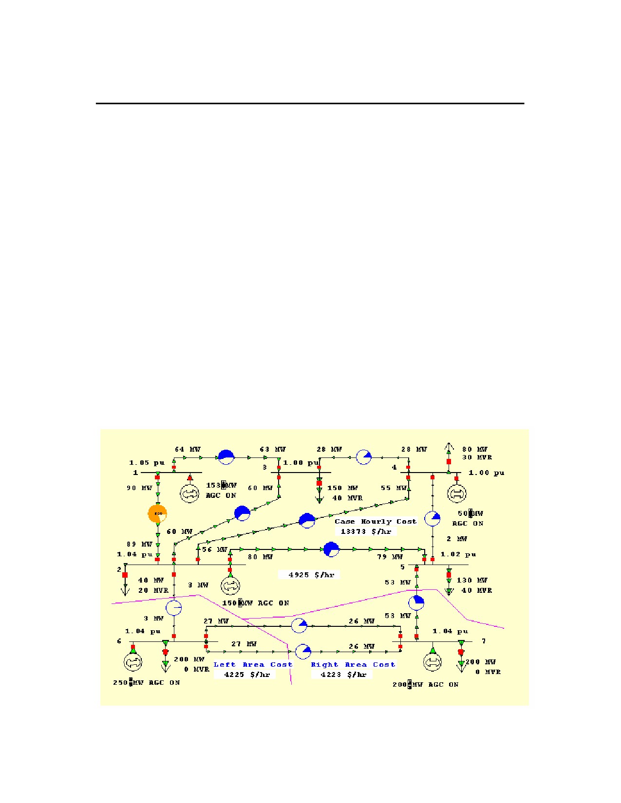
In this section we introduce an example of using the SCOPF. Consider the seven bus, three area system contained in
the file B7SCOPF (included with the PowerWorld Simulator). This case is the same case used in the OPF example,
except that the line from bus 2 to 3 has now a 100MVA rating, lines 1 to 2, 1 to 3 and 2 to 5 have a 120MVA rating,
and all three areas are initially on OPF control. To initially solve the case using the optimal power flow, select Primal
LP under LP OPF. The solution obtained is shown in Figure 1. The total case hourly cost is $ 13,372 / hr.
We are interested in determining an optimal solution that meets security constraints under contingency conditions. In
order to show that the current OPF solution does not enforce contingency violations, take line 1 to 2 out of service by
clicking in a circuit breaker. Then solve the power flow by pressing the Single Solution button. The result in Figure 2
indicates that line 1 to 2 is overloaded 32%. The SCOPF algorithm will attempt to move the operating solution such
that no contingency violation occurs in the system. Close line 1 to 2 back in service.
The next step is to specify the contingency conditions that the system should withstand. In order to do that, we access
the Contingency Analysis dialog under Tools . Note that we can also access this dialog from the SCOPF control
dialog by selecting LP OPF > Security Constrained OPF and pressing the View Contingency Analysis Form button
on the Options page. The B7SCOPF case does not have contingencies assoc iated with it. Insert single line
contingencies in the contingency list by pressing the Auto Insert button located at the bottom left of the Contingency
Analysis dialog. in the Auto Insert Dialog select the option for Single Transmission Line and select Numbers under
the Identify buses by field. Select Do Insert Contingencies. This will prompt to insert 11 single line contingencies
corresponding to all the lines in the system. Select Yes. You can now close the Contingency Analysis dialog.
Return to the Security Constrained Optimal Power Flow Form. You can set the SCOPF to use the OPF solution as
the base by selecting Solve base case using optimal power flow .
You can now solve the SCOPF by pressing the Run Full Security Constrained OPF. This will process the
contingency violations and iteratively solve the LP program and the power flow equations to minimize the objective
function and enforce equality and inequality constraints. The solution is shown in Figure 3. The total operating cost is
now $ 13,409. The increase in operating cost is due to enforcing security constraints. If a new contingency analysis is
performed using the optimal solution as the reference, it will be found that no contingency violations occur for the
contingencies in the list, i.e., branch flows are less than (or equal to) 100% in the post contingency condition. Thus,
the system meets all the specified constraints. You can analyze the SCOPF results by browsing the information in the
SCOPF tabs. Note that the CTG Constraints dialog does not show unenforceable constraints, but the branch
violation of line 2 to 5 due to the contingency 5 to 7 is now binding.
B7SCOPF Case Solved using OPF
723

B7SCOPF Power Flow Solution with line 1-2 open
B7SCOPF Case Solved using SCOPF: The system now meets the contingency constraints.
724

PowerWorld Simulator Add-on Tools
SCOPF Example: Marginal Prices
Using the SCOPF solution from the previous page, select the Bus Marginal Price Details from the Results page of
the SCOPF Dialog to view the detail of the marginal price components. Note in the following Figure that each area
constraint contributes equally to the marginal cost of the buses in that area. The binding inequality constraint from bus
2 to 5 makes further contribution to the bus marginal price of buses in area Top.
Seven Bus Case SCOPF Bus Marginal Price Details
725

SCOPF Example: Unenforceable Constraints
Using the same example as above, reduce the MVA rating of line 2 to 5 to 90 MVA. The initial base case LP OPF
solution is the same as in the previous example. Consider the same contingency list. When the contingencies are
solved using the initial OPF solution as the reference, seven contingency violations need to be removed. The CTG
dialog after simulation is presented in the following figure.
CTG Dialog after SCOPF Solution
We note that the constraint from bus 2 to 5 under a contingency from 5 to 7 is unenforceable. There are not enough
system controls to enforce the contingency constraint. A $ 1,000 / hr cost is assigned to unenforceable constraints in
this case. The cost of not enforcing constraints can be specified in the OPF Constraint Options Dialog.
726
PowerWorld Simulator Add-on Tools
Available Transfer Capability (ATC) Analysis
The ATC Analysis tool is only available if you have purchased the ATC add-on to the base Simulator package.
Contact PowerWorld Corporation for details about ordering the ATC version of Simulator.
Available Transfer Capability (ATC) analysis determines the maximum MW transfer possible between two parts of a
power system without violating any limits. Most often, this transfer is between two areas in the system.
Simulator’s ATC analysis makes use of several tools that are available elsewhere in Simulator. These include
· Power Transfer Distribution Factors (PTDFs): determine the linear impact of a transfer (or changes in power
injection) on the elements of the power system.
· Line Outage Distribution Factors (LODFs): determine the linear impact of a line outage on the elements of the
power system.
· Contingency Analysis: studies the impact of a list of contingencies on the power system.
· Limit Monitoring Settings: control which elements of the system are monitored for limit violations.
You do not directly use these other tools when using Simulator’s ATC analysis tool, but Simulator uses the settings
and algorithms in the background to determine ATC. Thus, it is helpful to be knowledgeable on their use, as it will help
you in interpreting the results of an ATC analysis.
· Simulator provides three methods of determining the ATC for a transfer direction. See : ATC Solution Methods
For information on how to use the Simulator ATC tool, see Available Transfer Capability Dialog.
727

ATC Dialog
Available Transfer Capability Dialog
The Available Transfer Capability Dialog provides you an interface for performing and viewing the results of
Available Transfer Capability Analysis. ATC analysis is typically only done on the present power system state or
scenario (called Single Scenario ATC Analysis). Click here for information on performing multiple scenarios analysis.
To open the ATC Dialog, select Tools > Available Transfer Capability (ATC) from the main menu. The dialog opens
to the Single Scenario ATC Analysis version with the Options tab, Common Options sub-tab visible. Click on any of
the desired tabs at the top of the dialog for more information on the contents of each.
ATC Dialog
The ATC Dialog is divided in three tabs: Options tab, Analysis tab, and Result tab. In addition, it has the following
controls:
Save/Load Settings
ATC Analysis settings can be saved by selecting Save Settings on the ATC dialog. This allows you to repeat the
analysis without having to reconfigure the settings. Select Load Settings to retrieve previously saved settings.
728
PowerWorld Simulator Add-on Tools
ATC Dialog: Options Tab
The Options Tab of the ATC Dialog is subdivided in three sub tabs: Common Options, Define Contingencies, and
Advanced Options. They have the following controls:
Common Options
Seller Type, Buyer Type
For the ATC Solution Method of Single Linear Step (SL), ATC can be calculated for transfers between combinations
of areas, zones, super areas, injection groups, buses, or to a slack bus. For other ATC Solution Methods, ATC can
be calculated for transfers between areas, super areas or injection groups only. Use the seller type and buyer type
options to indicate the type of the selling and purchasing entities.
Seller, Buyer
These dropdown boxes allow you to select the selling and buying entities. The contents of each depend on the
Seller/Buyer Types selected. Clicking the Find Seller and Find Buyer buttons allows you to use Simulator’s
Advanced Search Engine to locate the desired entities.
Reverse Buyer/Seller Button
Click this button to reverse the direction currently shown. The buyer becomes the seller, and the seller the buyer.
Linear Calculation Method
The ATC analysis tool can use either a Lossless DC or Lossless DC with Phase Shifters calculation method for
obtaining the ATC results.
If you select the Lossless DC option, branch flow sensitivity is calculated by estimating the real power that flows
through the monitored element only from the differenc e in angles measured across its terminals.
The Lossless DC with Phase Shifters method, a modification to the lossless dc approximation, takes into account
phase shifter operation. It is especially useful when the ATC tool continually reports overloads on branches that
obviously will not overload because of the operation of a phase shifting transformer.
The Linearized AC method is not yet available.
Include Contingencies Check Box
Check this box to include contingencies (inserted or loaded using the Contingency Analysis Tool) in the ATC
analysis. Note that minimizing the number of contingencies considered greatly improves solution speed as well as
computer memory requirements for doing ATC Analysis. Therefore, be careful in choosing which contingencies to
use with the ATC tool.
Report Base Case Limitations Check Box
When checked, the ATC tool will report transfer limitations from the base case.
Report Generation Reserve Limitations Check Box
When checked, the ATC tool will report transfer limitations from generation reserve.
Limit Monitoring Settings Button
Click this button to open the Limit Monitoring Settings Dialog. Note that minimizing the number of monitored power
system elements greatly improves solution speed as well as computer memory requirements for doing ATC
Analysis.
Transfer Results Reporting Options
Transfer Limiters to Save
This value tells Simulator how many total "Transfer Limiters" to save. Simulator will save those Transfer
Limiters with the lowest Transfer Limitation. An explanation of a Transfer Limiter follows
During Linear ATC Analysis, Simulator determines the "Transfer Limitation" (See Available Transfer Capability
Analysis) for each transmission line and interface during each contingency and the base case. From this
Simulator develops a list of Transfer Limiters. A Transfer Limit contains three pieces of information
· Transfer Limit in MW
· Transmission branch (or interface) that causes the limit
· Contingency that is applied to cause the limit (if it’s a limit without any contingency applied, then the
contingency will say "Base Case")
Thus if we are monitoring 1000 transmission lines during 99 contingencies plus 1 base case, there would be
100,000 Transfer Limiters calculated. We are not concerned with all 100,000 limitations, theref ore, only the
limitations with the smallest Transfer Limit in MW are reported.
729
Max Limiters per CTG
When analyzing a long list of contingencies, the worst transfer limitations may all occur during the same
contingency. Set this value to limit the number of Transfer Limiters saved that are associated with one
contingency.
Max Limiters per Element
Also, when analyzing a long list of contingencies, the worst transfer limitations may all be overload the same
limiting element. Set this value to limit the number of Transfer Limiters saved that are associated with one
Limiting Element.
Max MW Limitation
This value defines the maximum transfer to report between the buyer and seller. Simulator will compute the
ATC analysis results until the transfer amount reaches the value in this field, and only report the results meeting
the other reporting criteria up to this MW limitation.
Ignore Elements with OTDFs below
Simulator will not report Transfer Limitations for elements with OTDF values (or PTDF values if there is no
Limiting Contingency) less than this user-specified value. The default value is 0.5%, meaning that for 100 MW
transfer, there would be only a 0.5 MW increase in flow on the Limiting Element.
As described in Available Transfer Capability (ATC), the transfer limitation functions involve dividing by the
PTDF or OTDF values for each branch or interface. This leads to two facts:
· The accuracy of the transfer limitation is less for lines that have very small PTDF or OTDF values.
· A very small PTDF or OTDF value means that the transfer has very little impact on the line anyway.
These two facts often result in Linear ATC analysis reporting inaccurate transfer limitations for lines that are
largely unaffected by the transfer. It is not uncommon to have a transfer limitation report an extremely negative
transfer limit (e.g. -1.9E28 MW). A branch which is overloaded by a very small percentage, but which has a
very small OTDF value often causes this. If the OTDF value is 0.001%, then a branch overloaded by 1 MW will
result in a tranfer limitation of -100,000 MW.
This motivates the usefulness of ignoring elements with small PTDFs.
Ignore Elements with PTDFs below
Simulator will not report Transfer Limitations for elements with PTDF values less than this user-specified value.
The default value is 0.5%.
Define Contingencies
The Define Contingencies tab is similar to the Contingencies Tab of the Contingency Analysis Dialog. The user can
insert, auto-insert, define and/or delete contingency records. See Contingency Analysis for detailed information on
defining contingencies.
Advanced Options
ATC Solution Method
One of the solution methods of determining the ATC for a transfer direction.
Define Extra Monitors
Simulators ATC tool determines the maximum amount of MW transfer between the buyer and seller. If you would
like to also determine the flow on additional lines or interfaces at the transfer levels determined by the ATC tool, you
can utilize Extra Monitors. Click the Define Extra Monitors button to open the ATC Extra Monitors Dialog.
Analyze Multiple Scenarios
Check Analyze Multiple Scenarios to perform ATC Analysis on several scenarios. See
ATC Dialog for Multiple Scenarios for more information on Multiple Scenario Analysis.
Model Reactive Power for Linear Methods By…
The linearized methods used in ATC are based only on the changes in real power MW in the system, thus an
assumption needs to be made about the reaction of the Mvar flows during the linear calculations. The choices are
Ignoring reactive power, Assuming constant voltage magnitude, or Assuming reactive power does not
change .
For Linear Methods, Allow Amp Limits by Assuming a Constant Voltage Magnitude
If checked, Simulator will allow converting MVA limits to Amp limits by assuming constant voltage magnitudes
based on the base case full AC load flow operating point just prior to the ATC linear calculations.
Transfer Calculation Methods
Note: The Transfer Calculation Options section is disabled if the Single Linear Step Solution Method is selected.
Transfer Tolerance
730
PowerWorld Simulator Add-on Tools
This is the tolerance used using the Iterated Linear Step or (IL) then Full CTG Solution methods. The default is
10.
Max. Iterations
This is the maximum number of iterations used in the Iterated Linear Step or (IL) then Full CTG Solution
methods. The default is 10.
When Iterating, Ignore Limiters below
This value indicates a minimum transfer value for reporting the ATC analysis results. Any ATC results below
this value will not be displayed. In general, you do not want to use this option, as you are interested in all
transfer limitations during various contingencies. However, sometimes you may wish to ignore ATC results
below 0, as a negative ATC result signifies a base case overload or limitation under the given contingency
condition, prior to any additional transfer in the defined seller to buyer direction.
Transfer Limiters to Iterate on
This is the number of transfer limiters to iterate on in the Iterated Linear Step or (IL) then Full CTG Solution
methods. The default is 1.
Power Flow Solution Options
This button brings up the Power Flow Solution Options Dialog.
Define Contingency Solution Options
Click this button to open the Contingency Solution Options Dialog.
Use Specific Solution Options For Contingencies
When checked, the ATC tool will use the solution options defined by pressing the "Define Contingency Solution
Options" button for contingency analysis. When not checked, all solutions will use the options defined by
pressing the "Power Flow Solution Options" button.
Enforce OPF Constraints
This only affects the Iterated Linear or (IL) then Full CTG Solution Methods. When Enforce OPF Constraints is
checked, Simulator solves the Optimal Power Flow after each transfer increase.
731

ATC Dialog: Analysis Tab
The Analysis Tab of the ATC Dialog is used to control the analysis process. The scrollable window displays a record
of user-initiated actions relating to the analysis.
Analysis Tab
The Analysis tab has the following controls:
Start Analysis
The Start Analysis button begins the ATC Analysis using the settings and options defined by the user in the ATC
Analysis Dialog. Progress of the ATC Analysis is shown in the scrollable pane of the ATC Dialog - Analysis Tab
window.
Abort Calculation
When using one of the iterative ATC Solution Methods, or while analyzing Multiple Scenarios, click this button to
Abort the calculation.
Note: This does not immediately abort the solution. Simulator must restore the system state before completing the
abort.
Show Log
Click this button to show the Power Flow Solution Message Log.
Restore Initial State
732
PowerWorld Simulator Add-on Tools
Click this button to restore the system state to the state when the dialog was first opened.
Increase Transfer
Click this button to open the Ramp Transfer Up dialog in order to increase (or decrease) the transfer level manually.
733

ATC Dialog: Result Tab
When performing ATC Analysis on a single system state, the Result Tab is visible. The Result Tab consists of two
sections: A Transfer Limiters Display and a Contingency Definition Display.
Result Tab
The Transfer Limiters Display contains tabbed sheets containing information on Branch, Interface, and Nomogram
Limiters. The user can also choose to display All Limiters. See Transfer Limiters for more information.
The Contingency Definition section displays information on the limiting contingency for selected transfer limiter if the
user checked Include Contingencies on the Common Options tab.
734
PowerWorld Simulator Add-on Tools
ATC Extra Monitors Dialog
Simulator’s ATC tool determines the maximum amount of MW transfer between the buyer and seller. If you would like
to also determine the flow on additional lines or interfaces at the transfer levels determined by the ATC tool, then you
can utilize ATC Extra Monitors. To open the Extra Monitors dialog, click the Define Extra Monitors button on the
Advanced Options tab of the ATC Analysis Dialog
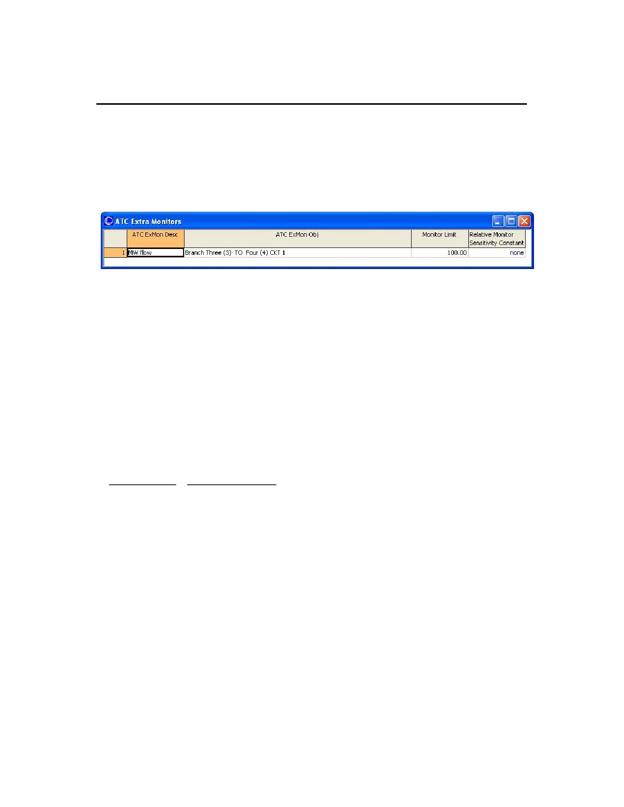
The ATC Extra Monitors Display lists all the ATC Extra Monitors defined. This list display is a Case Information
Display, and therefore has the same functionality as other common displays. See Adding and Removing Extra
Monitors.
Extra Monitors Dialog
The default fields shown on this display are:
ATC ExMon Desc
This is a description of the monitored value. Presently, this is always MW flow.
ATC ExMon Obj
The power system element that is being monitored. This will be either a transmission branch or an interface.
Monitor Limit
This is the MW limit of the element being monitored.
Relative Monitor
Set this to a positive value to further filter the Transfer Limitations reported on the Transfer Limiters Display. By
default, relative Monitor is set to none, and no additional filtering of limitations is performed. If this value is greater
than zero, then only Transfer Limitations that meet the following condition are included in the results.
OTDF
ExtraMon Rating
ELEMENT
¥
³
RelativeMonitor
PTDFELEMENT
Element Rating
This provides a measure of how much an interface or branch is affected by the transfer relative to its MW limit.
Adding and Removing Extra Monitors
To delete an extra monitor, right-click on the desired record on the list display and select Delete .
To insert an Extra Monitor, right-click on the list display and select Insert. This opens the insert dialog.
735
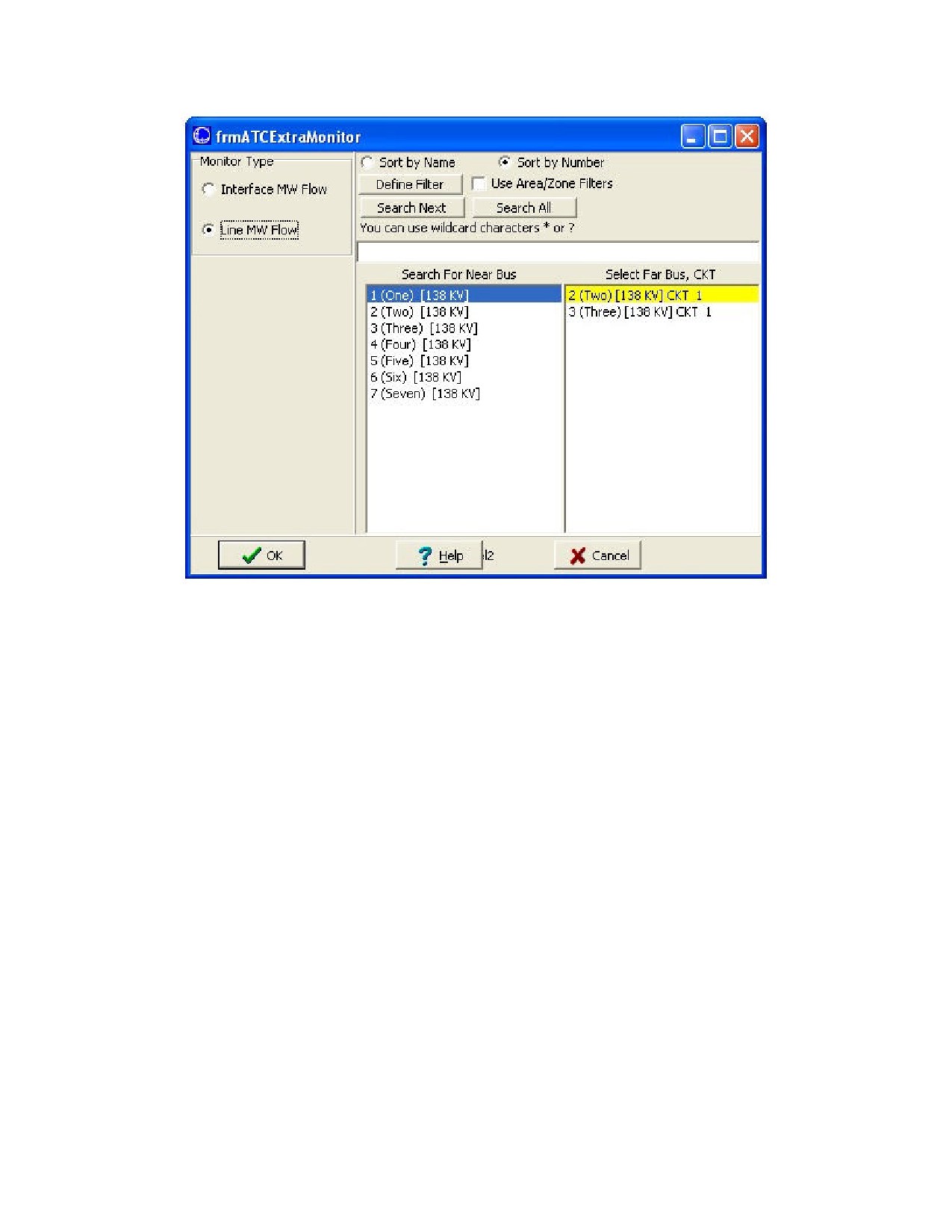
Insert Extra Monitors Dialog
Choose whether you want to monitor an Interface or Line MW flow. Next choose the interface or branch to be
monitored. Note that the insert dialog alllows the use of Simulator’s Advanced Search Engine and Filtering techniques
to aid in locating the desired interface or branch. Click OK to insert the record.
736

PowerWorld Simulator Add-on Tools
Multiple Scenario Available Transfer Capability Dialog
To perform Available Transfer Capability Analysis for several system scenarios, check Analyze Multiple Scenarios on
the Advanced Options tab of the Available Transfer Capability Dialog. When Analyze Multiple Scenarios is not
checked the available tabs are Options, Analysis and Result. When Analyze Multiple Scenarios is checked then the
following changes occur:
· Scenarios Tab appears
· Results Tab appears
· Result Tab is removed (replaced by Results)
Analyze Multiple Scenarios Dialog
By defining multiple scenarios, Simulator allows you to calculate ATC values for several different power system states
automatically. Scenarios can be modified along three axes:
· Line Rating/Zone Load Scenarios (weather-related scenarios)
· Generation Scenarios (generation profiles)
· Interface constraints
See Scenarios Tab for more information.
737

Multiple Scenario ATC Dialog: Scenarios Tab
By defining multiple scenarios, Simulator allows you to calculate ATC values for several different power system states
automatically. Scenarios can be modified along three axes:
· Line Rating/Zone Load Scenarios (weather-related scenarios)
· Generation Scenarios (generation profiles)
· Interface constraints
Analyze Multiple Scenarios Dialog: Scenarios Tab
Each tab contains a list of the power system elements that will be modified during different scenarios. These lists are
a familiar Case Information Display providing the same functionality as other displays
To insert a new power system element into the list, right click on the list (below the headings) and choose Insert.
On each tab, you may enter how many different scenarios should be defined for that kind of power system element.
For instance if you set Generation Scenarios to 5, then list display on the Generation Tab will provide 5 columns
labeled G0, G1, G2, G3, and G4. Generation outputs should then be entered into each cell representing the
generation output in each scenario.
Once you have specified the scenarios, Simulator is able to perform ATC Analysis on every combination of the axes.
For example, assume you have the following:
·
10 sets of line ratings and zones load
·
8 sets of generation profiles
738
PowerWorld Simulator Add-on Tools
·
3 interface constraints
This yields a total of 240 different scenarios to calculate (10*8*3 = 240 ). Be warned that that the more scenarios you
analyze the longer the computation will take.
Line Ratings and Zone Loads are varied together when analyzing scenarios. This was chosen because they often
vary together as a function of the weather. Notice that two sub-tabs (labeled Line Ratings and Zone Loads
respectively) appear at the bottom of the Line Ratings/Zone Loads tab.
The Scenarios Tab has the following controls:
Tabs and Sub-Tabs
The Scenarios Tab contains three tabbed sheets: Line Ratings/Zone Loads, Generator Outputs and Interface
Ratings.
Line Ratings and Zone Loads are varied together when analyzing scenarios. This was chosen because they often
vary together as a function of the weather. Notice that two sub-tabs (labeled Line Ratings and Zone Loads
respectively) appear at the bottom of the Line Ratings/Zone Loads tab.
Number of Defines Scenarios per Element Type
On each tab, you may enter how many different scenarios should be defined for that kind of power system element.
For instance if you set Generation Scenarios to 5, then list display on the Generation Tab will provide 5 columns
labeled G0, G1, G2, G3, and G4. Generation outputs should then be entered into each cell representing the
generation output in each scenario.
Total Scenarios
Once you have specified the scenarios, Simulator is able to perform ATC Analysis on every combination of the
axes. For example, assume you have the following:
·
10 sets of line ratings and zones load
·
8 sets of generation profiles
·
3 interface constraints
This yields a total of 240 different scenarios to calculate (10*8*3 = 240 ). Be warned that that the more scenarios
you analyze the longer the computation will take.
Set Scenario Names
This button will bring up the Scenario Names dialog, where the user is able to assign a different name to the
scenarios.
Assume Constant Power Factor
This option is only available in the Zone Loads sub-tab of the Line Ratings/Zone Loads tab. If selected, it specifies
that the Mvar will be ramped as the load MW are ramped, maintaining a constant power factor.
No Change in MVAR
This option is only available in the Zone Loads sub-tab of the Line Ratings/Zone Loads tab. If selected, it specifies
that the Mvar are kept constant, independently of the variations of the load MW.
Modified Elements
Each tab contains a list of the power system elements that will be modified during different scenarios. These lists
are a familiar Case Information Display providing the same functionality as other displays.
To insert a new power system element into the list, right click on the list (below the headings) and choose Insert.
739

Multiple Scenario ATC Dialog: Results Tab
Once you have defined your scenarios and started the ATC Analysis, you can switch to the Results Tab to see the
progress that ATC Analysis is making. Click on the diagram below for specific information on the contents of the
Results Tab.
Multiple Scenario Results Tab
The primary part of the Results tab contains a spreadsheet-like look-up table display. The layout of the display is
dictated by the Axis Order selected. See Local Menu Options for information regarding the Results Tab local menu.
This dialog has the following controls:
Show Transfer Limiters Button
Click the Show Transfer Limiters button to view the Transfer Limiters found under each scenario. This will open a
separate dialog that displays a list of the Transfer Limiters. To see the Transfer Limiters for a particular scenario,
click on the workbook cell that represents the scenario you are interested in and the separate dialog will update
appropriately.
Axis Order
This menu is used to select the desired axis order. The three axes correspond to the three Scenarios Tabs.
· One axis has heading labels G0, G1, … for the Generation Scenarios,
· Another with heading labels RL0, RL1, … for the Rating/Load Scenarios,
· A third with heading labels I0, I1, … for the Interface Scenarios.
740
PowerWorld Simulator Add-on Tools
Results Display
The primary part of the Results tab contains a spreadsheet-like look-up table display.
Write to Excel
This button will send the results to an Excel spreadsheet.
Save to Text Files
This option will allow the user to save the results in an auxiliary file.
741
Multiple Scenario ATC Analysis - Results Tab: Local Menu Options
If you right click on the workbook, you will bring up a local menu containing several options. The first several options
are only enabled if you right click on a cell representing a scenario. These options will perform an operation with
respect to the Scenario:
Take me to Scenario …
Will make modifications to the system state to take you to the Scenario.
Determine Transfer Limit For Scenario …
Will calculate the ATC for the Scenario, and then take you back to the Initial State.
Take me to the Transfe r Limit For Scenario …
Will perform ATC for the Scenario, and then ramp the transfer to this limit.
Other options on this local menu are not related to the Scenario you have clicked on.
Increase Transfer for Present System State
Will increment the transfer level for the present system state by a user-defined amount.
Return to Initial State
Will return the system state to the Initial State.
742

PowerWorld Simulator Add-on Tools
Transfer Limiters Display
The Transfer Limiters Display shows the results of ATC Analysis. This display appears either on the Result Tab of the
Available Transfer Capability Dialog or as a separate window when performing Multiple Scenario Available Transfer
Capability Analysis.
The display contains four different tabs: All Limiters, Branch Limiters, Interface Limiters, and Nomogram Interface
Limiters. Click the respective tabs below to find more information on each.
The list displays shown on each tab are instances of Case Information Displays. The default fields displayed are
shown below. Click on the respective columns on the list display below to view specific information about the display
fields.
The Contingency Definition Display at the bottom of the window shows information on the defined contingency that
caused the limitation selected from one of the four tabbed pages of limiters. For more information on this display, see
Contingency Analysis - Contingency Definition Display.
Transfer Limiters Display
The Transfer Limiters Display has the following controls:
All Limiters Tab
The All Limiters tab shows a list of all the transfer limitations found. This includes limitations on branches,
interfaces, areas, zones, etc…
Branch Limiters Tab
The Branch Limiters tab only shows those limitations with a transmission line or transformer as the limiting element.
The limiting element description for the Branch Limiters tab is replaced by the bus numbers and names of the
limiting element.
Interface Limiters Tab
The Interface Limiters Tab only shows those limitations with an interface as the limiting element. The limiting
element description is replaced by the name of the interface.
Nomogram Interface Limiters Tab
The Nomogram Interface Limiters Tab only shows those limitations with a nomogram interface as the limiting
element. The limiting element description is replaced by the name and segment of the nomogram interface.
Limiters Fields
Transfer Limiter Field
The Transfer Limit Field shows the Transfer Limit in MW for the Limiting Element during the Limiting
Contingency. This value depends on the ATC Solution Method Used:
· Single Linear Step (SL): Only Only one Linear ATC step is performed. The Transfer Limitation values are
those found during this step.
743
· Iterated Linear Step (IL): The Linear ATC method is iterated during this method. The Transfer Limiters
shown are those found during the final step performed. The actual Transfer Limitation values are the
values found at the last step plus the accumulated amount the transfer has been ramped. The Transfer
Limitation(s) that were used when iterating are highlighted in cyan.
· Iterated Linear Step (IL) then Full CTG: The Transfer Limiters shown are those found during the last
contingency analysis step that found violations. The Transfer Limitation values equal the accumulated
amount the transfer was ramped. Note that when performing the Full CTG Solution, negative ATC values
will not be probed, so the Transfer Limit will appear as 0 if there are violations in the Initial State. Any
Transfer Limiters that result in unsolvable contingencies are solved with the Single Linear step (SL) and
are highlighted in yellow .
Limiting Element Field
Shows a text description of the limiting element.
Limiting CTG Field
Shows the name of the limiting contingency.
% OTDF Field
This is the OTDF (or PTDF if the Limiting CTG is Base Case) on the Limiting Element for the transfer direction
that is being studied. In other words, this is a linear estimate of the percent of the transfer that will appear on
the Limiting Element if the Limiting CTG occurs.
Note: For Iterated Linear, this is the PTDF or OTDF at the last Linear Iteration. When using Full CTG Solution
Method, this is not calculated and will appear as 0 for all Limiters.
Pre-Transfer Value Estimate Field
If a contingency is not included in the Limiter, this is equal to the Initial Value. When a contingency is included
in the Limiter, this is the linear estimate of the post-contingency flow before any transfer occurs. See Available
Transfer Capability Analysis.
Note: For Iterated Linear, this is the estimate at the last Linear Iteration. When using (IL) Full CTG, this is not
calculated and will appear as 0 for all Limiters.
Limit Used Field
This is the value of the Limit being used by the ATC for the Limiting Element during the Limiting CTG. It reflects
what is specified in Limit Monitoring Settings.
Contingency Definition Display
This display shows information on the defined contingency that caused the limitation selected from one of the four
tabbed pages of limiters. For more information on this display, see Contingency Analysis - Contingency Definition
Display.
744
PowerWorld Simulator Add-on Tools
ATC Analysis Methods
ATC Analysis Methods - Solution Methods
Simulator provides three methods of determining the ATC for a transfer direction.
· Single Linear Step (SL)ATC_Analysis_Methods_Single_Linear_Step_SL_
· Iterated Linear Step (IL)ATC_Analysis_Methods_Iterated_Linear_Step_IL_
· Iterated Linear Step (IL) then Full CTGATC_Analysis_Methods_Iterated_Linear_Step_IL_then_Full_CTG_Solution
745
ATC Analysis Methods - Single Linear Step (SL)
The Single Linear Step approach is the most common ATC method and duplicates the ATC analysis done by many
system reliability organizations throughout North America. This method of ATC analysis uses only information about
the present system state and sensitivities (mathematical derivatives) about the present system state. These
sensitivities are embodied in the PTDF and LODF calculations.
Consider a transmission line with a limit of 10, present loading of 5 and a PTDF of 10%. The estimated maximum
transfer without causing on overload on line is
Transfer Limitation = (Limit - Present Loading) / PTDF = (10 - 5) / 0.1 = 50 MW
When including contingency analysis, the OTDF (Outage Transfer Distribution Factor) and linearized estimates of
post-contingency flows are used to determine the Transfer Limitation.
Transfer Limitation = (Limit - Post-Contingency Loading) / OTDF
If we find the Transfer Limitation for every transmission branch (and interface) during each contingency, then the ATC
is equal to the smallest Transfer Limitation.
Note: Simulator also monitors the possibility that a transfer will reduce the flow on a line until the line reaches its limit
for flow in the opposite direction.
746
PowerWorld Simulator Add-on Tools
ATC Analysis Methods - Iterate d Linear Step (IL)
The Single Linear Step is an extremely fast method for determining the ATC. However, because it only uses present
operating point information, controller changes are not taken into account. The linearization assumes that all
controllers are fixed. The Iterated Linear Step (IL) method provides an alternative to the Single Linear Step, but still
performs its analysis in a reasonable amount of time. The (IL) method operates as follows
· Stepsize = ATC using Single Linear Step (Note: save this initial step size for use by the Full CTG Solution)
· If [abs(stepsize) < Tolerance] then stop
· Ramp transfer out an additional amount of Stepsize and resolve Power Flow
· At new operating point, Stepsize = ATC using Single Linear Step
· Go to step 2
This method takes into account controller changes that occur as you ramp out to the transfer level, but still avoids the
full simulation of contingencies.
This method can be applied between combinations of areas and super areas, OR between two injection groups.
Combinations of areas/superareas and injection groups are not allowed.
747
ATC Analysis Methods - Iterated Linear Step (IL) then Full CTG Solution
If you want to absolutely test the validity of the ATC number, then you can use this method. Be aware however, that
this calculation method can be extremely slow. The (IL) then Full CTG Solution method operates as follows.
1 Run Iterated Linear Step and ramp transfer out ATC Value found
2 Stepsize = 10% of the initial Linear Step Size saved during the (IL) method, or 50 MW whichever is larger.
3 Run Full Contingency Analysis on the ramped transfer state
4 If there are violations then change the sign of Stepsize
5 if [abs(stepsize) < Tolerance] then Stop
6 Ramp transfer out an additional amount of Stepsize and resolve Power Flow
7 At new operating point, Run Full Contingency Analysis
8 IF [ (Stepsize > 0) AND (Violations) OR (Stepsize < 0) AND (NO Violations) ]
THEN Stepsize := -Stepsize/2 (switch direction)
9 Go to step 5
This method can be applied between combinations of areas and superareas, OR between two injection groups.
Combinations of areas/superareas and injection groups are not allowed.
748
PowerWorld Simulator Add-on Tools
Simulator Automation Server (SIMAUTO)
Simulator Automation Server (SimAuto) Overview
:
The SimAuto tool is only available if you have purchased the SimAuto add-on to the base Simulator package.
Contact PowerWorld Corporation for details about ordering the SimAuto version of Simulator.
PowerWorld Corporation also offers Optimal Power Flow (OPF), Available Transfer Capability ATC, Simulation
Automation Server (SimAuto), and Security Constrained Optimal Power Flow (SCOPF) add-ons. For more information
see PowerWorld Simulator Add-On Tools.
SimAuto provides PowerWorld customers the ability to access PowerWorld Simulator functionality within a program
written externally by the user. The Simulator Automation Server acts as a COM object, which can be accessed from
various programming languages that have COM compatibility. Examples of programming tools with COM compatibility
are Borland‚ Delphi, Microsoft‚ Visual C++, Microsoft‚ Visual Basic, and Matlab‚ (among others). For more
information on COM Objects and Automation Servers, see the help for Microsoft Windows.
The Automation Server of Simulator works very well in combination with Simulator Script Commands and Auxiliary
Files. It is beneficial to become familiar with these topics when considering using the Simulator Automation Server.
Note that previous users of SimAuto in Version 9 will need to update their function calls to SimAuto functions.
PowerWorld Corporation found it imperative to change the function calls for SimAuto, in order to remedy irreconcilable
problems when using SimAuto with some programming languages. The documentation provided should provide
adequate help on the changes needed, but as always, if any questions arise, please contact PowerWorld Corporation
for more information.
749
Starting Simulator Automation Server
Installing Simulator Automation Server
:
Note that previous users of SimAuto in Version 9 will need to update their function calls to SimAuto functions.
PowerWorld Corporation found it imperative to change the function calls for SimAuto, in order to remedy irreconcilable
problems when using SimAuto with some programming languages. The documentation provided should provide
adequate help on the changes needed, but as always, if any questions arise, please contact PowerWorld Corporation
for more information.
Installing the Simulator Automation Server requires no additional steps beyond installing PowerWorld Simulator as
normal. When a version of PowerWorld Simulator containing the Simulator Automation Server is installed on your
computer, the install program automatically adds the information needed by the Simulator Automation Server to the
registry.
If for some reason the registration fails, be sure you have the SimAuto add-on for Simulator and you have either run
the application on the computer or run the command pwrworld / regserver at the command line. If instead you would
like SimAuto to un-register itself as a COM object, run the command pwrworld /unregserver at the command line.
750
PowerWorld Simulator Add-on Tools
Including Simulator Automation Server Functions
:
Before you can access the functions defined by the Simulator Automation Server when writing the code for your
external program, you must first include the library of functions defined for the Simulator Automation Server. This kind
of library is referred to as a Type Library, which describes the available functions in a manner that can be interpreted
by different programming languages. Importing a Type Library from another program is usually fairly simple, but the
procedure does vary depending on the programming tool you are using. Please see the help for your programming
tool of choice on how to import a Type Library or COM functions from another program.
Examples
The following examples are just a few specific examples for certain programming media. The procedure may be
different for other programming media not listed. In addition, a procedure given for a certain type of programming
media may be one variation from several possible procedures for accomplishing the same task.
Borland Delphi
· Install the version of PowerWorld Simulator with the Simulator Automation Server included.
· In Delphi, choose Import Type Library… from the Project menu.
· In the list of libraries, search for and choose pwrworld Library.
· If pwrworld Library is not in the list, click Add. Find and choose the Pwrworld.exe file from the PowerWorld
Simulator directory, and click Open.
· You should see the class name TSimulatorAuto in the list of Class names.
· Click Install to include the PowerWorld Simulator Type Library.
Microsoft Visual Basic for Applications
· No additional tasks are necessary
· Importing Type Library still works (See Including Functions for version 9).
Microsoft Visual C++
· Install the version of PowerWorld Simulator with the Simulation Automation Server included.
· Add #import "…\powerworld.exe" in your external program code, using the full path to the PowerWorld
Simulator executable program.
· Add using namespace pwrworld in your external program code.
Matlab v.6.5 r.13
· No additional tasks are necessary.
751
Connecting to Simulator Automation Server
:
Once the Type Library or COM functions have been included in your programming environment, the Simulator
Automation Server can be handled as any other object in your code. The method for assigning and connecting to the
Simulator Automation Server can vary depending on the programming environment used, but the idea is basically the
same. You define a variable in your program to point to the server object, which is called SimulatorAuto. If the Type
Library was imported properly, you should have full access to the SimulatorAuto object and its defined functions.
Again, the procedure for creating the object and connecting to SimulatorAuto may vary for different programming
languages. Check the help for your programming environment on connecting to COM or Automation servers.
Examples
The following examples are just a few specific examples for certain programming media. The procedure may be
different for other programming media not listed. In addition, a procedure given for a certain type of programming
media may be one variation from several possible procedures for accomplishing the same task.
Borland Delphi 5
· Add pwrworld_TLB to the uses section of your unit.
· Declare a variable globally or as part of another object: A : ISimulatorAuto
· Initialize the variable: A := nil
· To connect to the Simulator Automation Server, create the connection: A := CoSimulatorAuto.create
· Perform function calls to the Simulator Automation Server: Output := A.SomeFunction(parameters)
· To close the connection to the Simulator Automation Server, remove the reference by again setting: A :=
nil
Microsoft Visual Basic for Applications
Early Binding:
· To connect to the Simulator Automation Server, create the connection initializing the variable:
Dim A as New pwrworld.SimulatorAuto
Late Binding:
· Declare a variable globally or as part of another object or function: Dim A As Object
· To connect to the Simulator Automation Server, create the connection:
Set A = CreateObject("pwrworld.SimulatorAuto")
Both Early and Late Binding:
· Perform function calls to the Simulator Automation Server: Output = A.SomeFunction parameters
· To close the connection to the Simulator Automation Server, remove the reference: Set A = Nothing
· If Type Library was imported, connection can also be achieved as in version 9 (See Connecting to
Simulator Automation Server in version 9).
Microsoft Visual C++
· Declare a variable globally or as part of another object or function: IsimulatorAutoPtr *A
· Declare a variable globally or as part of another object or function: CLSID clsid
· Declare a variable globally or as part of another object or function: HRESULT hr
· Obtain the class identifier (clsid) with the following command:
hr = CLSIDFromProgID(L"pwrworld.SimulatorAuto", &clsid)
· Initialize variable A: A = new IsimulatorAutoPtr
· To connect to the Simulator Automation Server, create the connection:
hr = A>CreateInstance(clsid, NULL, CLSCTX_SERVER)
· Perform function calls to the Simulator Automation Server: Output = A.SomeFunction(parameters)
· To close the connection to the Simulator Automation Server, release the reference:
hr = A>Release()
Matlab v.6.5 r.13
· To connect to the Simulator Automation Server, create the connection:
752
PowerWorld Simulator Add-on Tools
A = actxserver(‘pwrworld.SimulatorAuto’)
· Perform function calls to the Simulator Automation Server: Output = A.SomeFunction(parameters)
· To close the connection to the Simulator Automation Server, delete the connection: delete(A)
753
Simulator Automation Server Functions
Passing Data to the Simulator Automation Server
:
Passing Data to the Simulator Automation Server
All data to the Simulator Automation Server is passed by value rather than by reference (in pointer terminology, this
corresponds to sending data instead of pointer to data; in Microsoft Visual Basic®, this corresponds to sending data
ByVal instead of ByRef). This makes the marshalling of data between client software and the COM object much
easier.
No Optional Parameters
There are no optional parameters for any of the Simulator Automation functions. All functions must be called with
every argument filled.
754
PowerWorld Simulator Add-on Tools
Getting Data from the Simulator Automation Server
The Output Structure
Every function called on the SimulatorAuto object returns the same value, Output, which has a well-defined structure.
Output is of type VARIANT, and is an array of VARIANT’s. Output is zero-indexed.
The first element always contains any errors occurring during execution. For those functions returning more than one
element in the Output array (e.g. ListOfDevices), explanation is provided below when discussing the specific method.
Error Handling
As mentioned above, the first item in the Output VARIANT array, Output[0], contains any errors occurring during the
function’s execution. If no errors occurred during the function’s execution, Output[0] will be set to an empty BSTR
(string) represented in most languages by either ‘’ or "".
Error Format
If an error string is returned, it will be in the following format:
[method name]: [error_explanation]
e.g. RunScriptCommand: Error occurred processing script command - check command syntax
755
Simulator Automation Server Functions
The following list of functions is currently available once the SimulatorAuto object is set in your code. Check the help
sections on these functions to see more detail on the particular function.
ChangeParameters
CloseCase
GetParametersSingleElement
GetParametersMultipleElement
GetParameters (for compatibility with version 9)
ListOfDevices
OpenCase
ProcessAuxFile
RunScriptCommand
GetFieldList
SaveState
LoadState
SaveCase
SendToExcel
WriteAuxFile
756
PowerWorld Simulator Add-on Tools
ChangeParameters Function
The ChangeParameters function allows you to set a list of parameters for a specific object in a case loaded into the
Simulator Automation Server. In addition to changing parameters for objects, this function can also be used to set
options for some of the Simulator tools, such as ATC and OPF. This function is identical in setup to the
GetParametersSingleElement function, with the exception that the Values array must contain a value for each field
variable given in the ParamList array.
Function Prototype
ChangeParameters(ObjectType, ParamList, Values)
Parameter Definitions
ObjectType : String
The type of object you are changing parameters for.
ParamList : Variant
A variant array storing strings (COM Type BSTR). This array stores a list of
PowerWorld‚ object field variables, as defined in the section on PowerWorld
Object Fields. The ParamList must contain the key field variables for the
specific device, or the device cannot be identified.
Values : Variant
A variant array storing variants. This array can store any type of information
(integer, string, etc.) in each array position. A value should be passed for each
field variable given in the ParamList. The Values array must contain the key
field values for the specific device, or the device cannot be identified.
Output
ChangeParameters only returns the first element in Output, the error string.
Notes
The ParameterList and Values arrays must be the same size, as each parameter must have a corresponding
value to be assigned.
757
ChangeParameters Function: Sample Code
Borland® Delphi
Var ParamList, ValueList : OLEVariant
// Set ParamList up to modify the maximum number of iterations
// and the system base for the power flow simulations
ParamList := VarArrayCreate([1,2], varOleStr);
ParamList[1] := 'MaxItr';
ParamList[2] := 'SBase';
// ValueList is setup with 41 and 410 for MaxItr and SBase,
// respectively
ValueList := VarArrayCreate([1,2], varOleStr);
ValueList[1] := 41;
ValueList[2] := 410;
// Make the ChangeParameters call
Output = SimAuto.ChangeParameters('Sim_Solution_Options', _
ParamList, ValueList)
Microsoft® Visual Basic for Applications
' Set ParamList up to modify the maximum number of iterations
' and the system base for the power flow simulations
Dim ParamList As Variant
ParamList = Array("MaxItr", "Sbase")
' ValueList is setup with 41 and 410 for MaxItr and SBase,
' respectively
Dim ValueList As Variant
ValueList = Array(45, 90)
' Make the ChangeParameters call
Output = SimAuto.ChangeParameters("Sim_Solution_Options", _
ParamList, ValueList)
Matlab®
% Set ParamList up to modify the maximum number of iterations
% and the system base for the power flow simulations
ParamList = {'MaxItr' 'Sbase'};
% values is setup with 41 and 410 for MaxItr and SBase,
% respectively
values = [41 410];
% Convert the values matrix to a set of cells for passing
% through the COM interface
ValueList = num2cell(values);
758