Content      ..     2      3      4      5     ..

ISO 32000-1 Document management — Portable document format — Part 1: PDF 1.7 - page 4

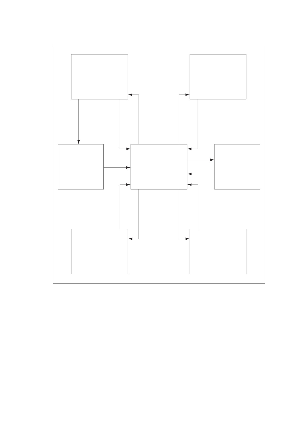
Path object

Text object

Allowed operators:

Allowed operators:

• Path construction

• General graphics state

• Color

• Text state

• Text-showing

• Text-positioning

• Marked-content

W,W* Path-painting

m, re

BT

ET

operators

Clipping path object

Page description level

Shading object

Allowed operators:

Allowed operators:

sh

Allowed operators:

• None

Path-painting

• General graphics state

• None

operators

• Special graphics state

• Color

(immediate)

• Text state

• Marked-content

EI

BI

Do

(immediate)

In-line image object

External object

Allowed operators:

Allowed operators:

• ID

• None

Figure 9 - Graphics Objects

EXAMPLE

The path construction operators m and re signal the beginning of a path object. Inside the path object,

additional path construction operators are permitted, as are the clipping path operators W and W*, but not

general graphics state operators such as w or J. A path-painting operator, such as S or f, ends the path

object and returns to the page description level.

NOTE

A conforming reader may process a content stream whose operations violate these rules for describing

graphics objects and can produce unpredictable behaviour, even though it may display and print the stream

correctly. Applications that attempt to extract graphics objects for editing or other purposes depend on the

objects’ being well formed. The rules for graphics objects are also important for the proper interpretation of

marked content (see 14.6, "Marked Content").

A graphics object also implicitly includes all graphics state parameters that affect its behaviour. For instance, a

path object depends on the value of the current colour parameter at the moment the path object is defined. The

effect shall be as if this parameter were specified as part of the definition of the path object. However, the

operators that are invoked at the page description level to set graphics state parameters shall not be

113

coordinates may increase from the top of the page to the bottom on some devices and from bottom to top on

others. Finally, different devices have different resolutions; some even have resolutions that differ in the

horizontal and vertical directions.

NOTE

If coordinates in a PDF file were specified in device space, the file would be device-dependent and would

appear differently on different devices.

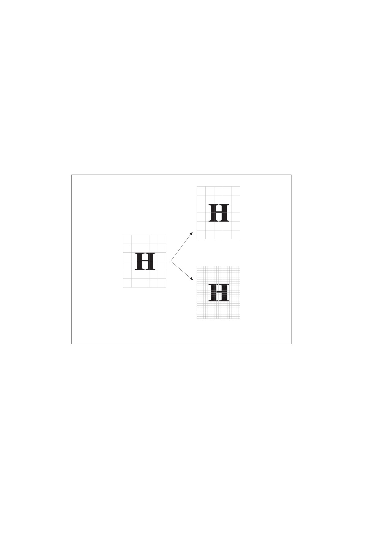
EXAMPLE

Images specified in the typical device spaces of a 72-pixel-per-inch display and a 600-dot-per-inch printer

would differ in size by more than a factor of 8; an 8-inch line segment on the display would appear less

than 1 inch long on the printer. Figure 10 in Annex L shows how the same graphics object, specified in

device space, can appear drastically different when rendered on different output devices.

Device space for

Device space for

72-dpi screen

300-dpi printer

Figure 10 - Device Space

8.3.2.3

User Space

To avoid the device-dependent effects of specifying objects in device space, PDF defines a device-independent

coordinate system that always bears the same relationship to the current page, regardless of the output device

on which printing or displaying occurs. This device-independent coordinate system is called user space.

The user space coordinate system shall be initialized to a default state for each page of a document. The

CropBox entry in the page dictionary shall specify the rectangle of user space corresponding to the visible

area of the intended output medium (display window or printed page). The positive x axis extends horizontally

to the right and the positive y axis vertically upward, as in standard mathematical practice (subject to alteration

by the Rotate entry in the page dictionary). The length of a unit along both the x and y axes is set by the

UserUnit entry (PDF 1.6) in the page dictionary (see Table 30). If that entry is not present or supported, the

default value of 1 ⁄ 72 inch is used. This coordinate system is called default user space.

NOTE 1

In PostScript, the origin of default user space always corresponds to the lower-left corner of the output

medium. While this convention is common in PDF documents as well, it is not required; the page dictionary’s

CropBox entry can specify any rectangle of default user space to be made visible on the medium.

NOTE 2

The default for the size of the unit in default user space (1⁄ 72 inch) is approximately the same as a point, a unit

widely used in the printing industry. It is not exactly the same, however; there is no universal definition of a

point.

Conceptually, user space is an infinite plane. Only a small portion of this plane corresponds to the imageable

area of the output device: a rectangular region defined by the CropBox entry in the page dictionary. The region

of default user space that is viewed or printed can be different for each page and is described in 14.11.2, "Page

Boundaries".

Coordinates in user space (as in any other coordinate space) may be specified as either integers or real

numbers, and the unit size in default user space does not constrain positions to any arbitrary grid. The

resolution of coordinates in user space is not related in any way to the resolution of pixels in device space.

115

The transformation from user space to device space is defined by the current transformation matrix (CTM), an

element of the PDF graphics state (see 8.4, "Graphics State"). A conforming reader can adjust the CTM for the

native resolution of a particular output device, maintaining the device-independence of the PDF page

description. Figure 11 in Annex L shows how this allows an object specified in user space to appear the same

regardless of the device on which it is rendered.

NOTE 3

The default user space provides a consistent, dependable starting place for PDF page descriptions regardless

of the output device used. If necessary, a PDF content stream may modify user space to be more suitable to its

needs by applying the coordinate transformation operator, cm (see 8.4.4, "Graphics State Operators"). Thus,

what may appear to be absolute coordinates in a content stream are not absolute with respect to the current

page because they are expressed in a coordinate system that may slide around and shrink or expand.

Coordinate system transformation not only enhances device-independence but is a useful tool in its own right.

EXAMPLE

A content stream originally composed to occupy an entire page can be incorporated without change as an

element of another page by shrinking the coordinate system in which it is drawn.

Device space for

72-dpi screen

CTM

User space

Device space for

300-dpi printer

Figure 11 - User Space

8.3.2.4

Other Coordinate Spaces

In addition to device space and user space, PDF uses a variety of other coordinate spaces for specialized

purposes:

•

The coordinates of text shall be specified in text space. The transformation from text space to user space

shall be defined by a text matrix in combination with several text-related parameters in the graphics state

(see 9.4.2, "Text-Positioning Operators").

•

Character glyphs in a font shall be defined in glyph space (see 9.2.4, "Glyph Positioning and Metrics"). The

transformation from glyph space to text space shall be defined by the font matrix. For most types of fonts,

this matrix shall be predefined to map 1000 units of glyph space to 1 unit of text space; for Type 3 fonts, the

font matrix shall be given explicitly in the font dictionary (see 9.6.5, "Type 3 Fonts").

•

All sampled images shall be defined in image space. The transformation from image space to user space

shall be predefined and cannot be changed. All images shall be 1 unit wide by 1 unit high in user space,

116

regardless of the number of samples in the image. To be painted, an image shall be mapped to a region of

the page by temporarily altering the CTM.

•

A form XObject (discussed in 8.10, "Form XObjects") is a self-contained content stream that can be treated

as a graphical element within another content stream. The space in which it is defined is called form space.

The transformation from form space to user space shall be specified by a form matrix contained in the form

XObject.

•

PDF 1.2 defined a type of colour known as a pattern, discussed in 8.7, "Patterns". A pattern shall be

defined either by a content stream that shall be invoked repeatedly to tile an area or by a shading whose

colour is a function of position. The space in which a pattern is defined is called pattern space. The

transformation from pattern space to user space shall be specified by a pattern matrix contained in the

pattern.

•

PDF 1.6 embedded 3D artwork, which is described in three-dimensional coordinates (see 13.6.5,

"Coordinate Systems for 3D") that are projected into an annotation’s target coordinate system (see 13.6.2,

"3D Annotations").

8.3.2.5

Relationships among Coordinate Spaces

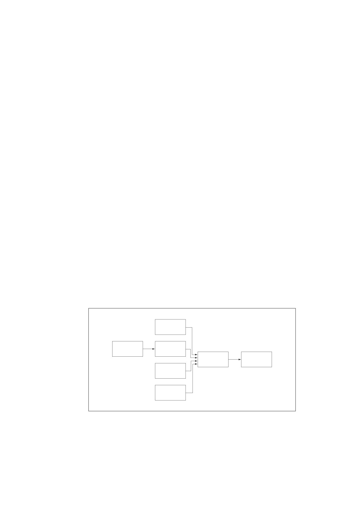
Figure 12 in Annex L shows the relationships among the coordinate spaces described above. Each arrow in the

figure represents a transformation from one coordinate space to another. PDF allows modifications to many of

these transformations.

Because PDF coordinate spaces are defined relative to one another, changes made to one transformation can

affect the appearance of objects defined in several coordinate spaces.

EXAMPLE

A change in the CTM, which defines the transformation from user space to device space, affects forms,

text, images, and patterns, since they are all upstream from user space.

8.3.3

Common Transformations

A transformation matrix specifies the relationship between two coordinate spaces. By modifying a

transformation matrix, objects can be scaled, rotated, translated, or transformed in other ways.

Form

space

Glyph

Text

space

space

User

Device

space

space

Image

space

Pattern

space

Figure 12 - Relationships Among Coordinate Systems

A transformation matrix in PDF shall be specified by six numbers, usually in the form of an array containing six

elements. In its most general form, this array is denoted

[a b c d e f ]; it can represent any linear

transformation from one coordinate system to another. This sub-clause lists the arrays that specify the most

common transformations;

8.3.4, "Transformation Matrices", discusses more mathematical details of

transformations, including information on specifying transformations that are combinations of those listed here:

117

•

Translations shall be specified as [ 1 0 0 1 t_x t_y ], where t_x and t_y shall be the distances to translate the

origin of the coordinate system in the horizontal and vertical dimensions, respectively.

•

Scaling shall be obtained by [ s_x 0 0 s_y 0 0 ]. This scales the coordinates so that 1 unit in the horizontal

and vertical dimensions of the new coordinate system is the same size as s_x and s_y units, respectively, in

the previous coordinate system.

•

Rotations shall be produced by [ cos q sin q -sin q cos q 0 0 ], which has the effect of rotating the

coordinate system axes by an angle q counter clockwise.

•

Skew shall be specified by [ 1 tan a tan b 1 0 0 ], which skews the x axis by an angle a and the y axis by

an angle b.

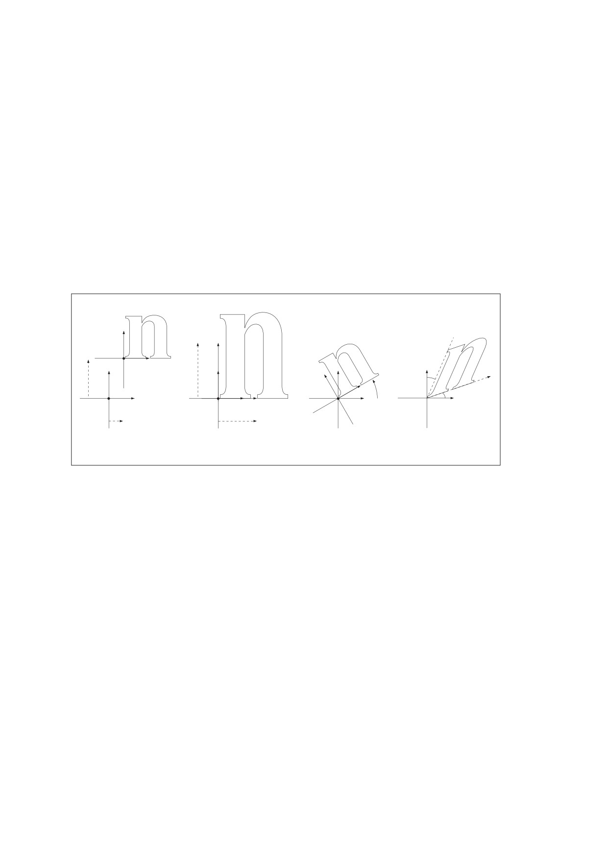
Figure 13 in Annex L shows examples of each transformation. The directions of translation, rotation, and skew

shown in the figure correspond to positive values of the array elements.

s_y

b

t_y

q

a

t_x

s_x

Translation

Scaling

Rotation

Skewing

Figure 13 - Effects of Coordinate Transformations

NOTE

If several transformations are combined, the order in which they are applied is significant. For example, first

scaling and then translating the x axis is not the same as first translating and then scaling it. In general, to

obtain the expected results, transformations should be done in the following order: Translate, Rotate, Scale or

skew.

Figure 14 in Annex L shows the effect of the order in which transformations are applied. The figure shows two

sequences of transformations applied to a coordinate system. After each successive transformation, an outline

of the letter n is drawn.

118

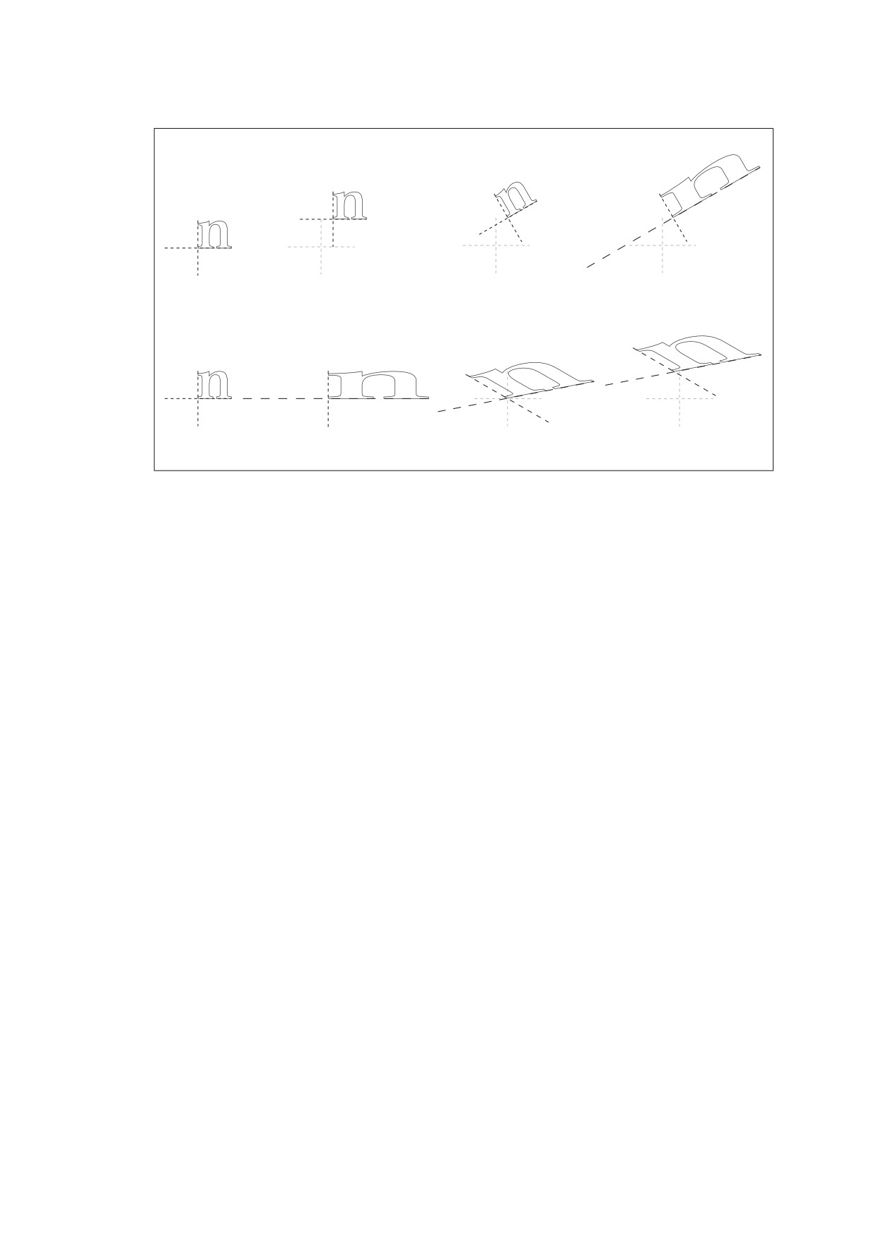
Original

Step 1: Translation

Step 2: Rotation

Step 3: Scaling

Original

Step 1: Scaling

Step 2: Rotation

Step 3: Translation

Figure 14 - Effect of Transformation Order

NOTE

The following transformations are shown in the figure: a translation of 10 units in the x direction and 20 units in

the y direction; a rotation of 30 degrees; a scaling by a factor of 3 in the x direction

In the figure, the axes are shown with a dash pattern having a 2-unit dash and a 2-unit gap. In addition, the

original (untransformed) axes are shown in a lighter colour for reference. Notice that the scale-rotate-translate

ordering results in a distortion of the coordinate system, leaving the x and y axes no longer perpendicular; the

recommended translate-rotate-scale ordering results in no distortion.

8.3.4

Transformation Matrices

This sub-clause discusses the mathematics of transformation matrices.

To understand the mathematics of coordinate transformations in PDF, it is vital to remember two points:

•

Transformations alter coordinate systems, not graphics objects. All objects painted before a transformation

is applied shall be unaffected by the transformation. Objects painted after the transformation is applied

shall be interpreted in the transformed coordinate system.

•

Transformation matrices specify the transformation from the new (transformed) coordinate system to the

original

(untransformed) coordinate system. All coordinates used after the transformation shall be

expressed in the transformed coordinate system. PDF applies the transformation matrix to find the

equivalent coordinates in the untransformed coordinate system.

NOTE 1

Many computer graphics textbooks consider transformations of graphics objects rather than of coordinate

systems. Although either approach is correct and self-consistent, some details of the calculations differ

depending on which point of view is taken.

PDF represents coordinates in a two-dimensional space. The point (x, y) in such a space can be expressed in

vector form as [ x y 1 ]. The constant third element of this vector (1) is needed so that the vector can be used

with 3-by-3 matrices in the calculations described below.

The transformation between two coordinate systems can be represented by a 3-by-3 transformation matrix

written as follows:

119

coordinates. Not all transformations are invertible, however. For example, if a matrix contains a, b, c, and d

elements that are all zero, all user coordinates map to the same device coordinates and there is no unique

inverse transformation. Such noninvertible transformations are not very useful and generally arise from

unintended operations, such as scaling by 0. Use of a noninvertible matrix when painting graphics objects can

result in unpredictable behaviour.

8.4

Graphics State

8.4.1

General

A conforming reader shall maintain an internal data structure called the graphics state that holds current

graphics control parameters. These parameters define the global framework within which the graphics

operators execute.

EXAMPLE 1

The f (fill) operator implicitly uses the current colour parameter, and the S (stroke) operator additionally

uses the current line width parameter from the graphics state.

A conforming reader shall initialize the graphic state at the beginning of each page with the values specified in

Table 52 and Table 53. Table 52 lists those graphics state parameters that are device-independent and are

appropriate to specify in page descriptions. The parameters listed in Table 53 control details of the rendering

(scan conversion) process and are device-dependent; a page description that is intended to be

device-

independent should not be written to modify these parameters.

Table 52 - Device-Independent Graphics State Parameters

Parameter

Type

Value

CTM

array

The current transformation matrix, which maps positions from

user coordinates to device coordinates (see 8.3, "Coordinate

Systems"). This matrix is modified by each application of the

coordinate transformation operator, cm. Initial value: a matrix

that transforms default user coordinates to device

coordinates.

clipping path

(internal)

The current clipping path, which defines the boundary against

which all output shall be cropped (see 8.5.4, "Clipping Path

Operators"). Initial value: the boundary of the entire

imageable portion of the output page.

color space

name or array

The current colour space in which colour values shall be

interpreted

(see

8.6, "Colour Spaces"). There are two

separate colour space parameters: one for stroking and one

for all other painting operations. Initial value: DeviceGray.

color

(various)

The current colour to be used during painting operations (see

8.6, "Colour Spaces"). The type and interpretation of this

parameter depend on the current colour space; for most

colour spaces, a colour value consists of one to four

numbers. There are two separate colour parameters: one for

stroking and one for all other painting operations. Initial value:

black.

text state

(various)

A set of nine graphics state parameters that pertain only to

the painting of text. These include parameters that select the

font, scale the glyphs to an appropriate size, and accomplish

other effects. The text state parameters are described in 9.3,

"Text State Parameters and Operators".

line width

number

The thickness, in user space units, of paths to be stroked

(see 8.4.3.2, "Line Width"). Initial value: 1.0.

121

Table 52 - Device-Independent Graphics State Parameters (continued)

Parameter

Type

Value

line cap

integer

A code specifying the shape of the endpoints for any open

path that is stroked (see 8.4.3.3, "Line Cap Style"). Initial

value: 0, for square butt caps.

line join

integer

A code specifying the shape of joints between connected

segments of a stroked path (see 8.4.3.4, "Line Join Style").

Initial value: 0, for mitered joins.

miter limit

number

The maximum length of mitered line joins for stroked paths

(see 8.4.3.5, "Miter Limit"). This parameter limits the length of

“spikes” produced when line segments join at sharp angles.

Initial value: 10.0, for a miter cutoff below approximately 11.5

degrees.

dash pattern

array and

A description of the dash pattern to be used when paths are

number

stroked (see 8.4.3.6, "Line Dash Pattern"). Initial value: a

solid line.

rendering intent

name

The rendering intent to be used when converting CIE-based

colours to device colours (see 8.6.5.8, "Rendering Intents").

Initial value: RelativeColorimetric.

stroke adjustment

boolean

(PDF 1.2) A flag specifying whether to compensate for

possible rasterization effects when stroking a path with a line

width that is small relative to the pixel resolution of the output

device (see 10.6.5, "Automatic Stroke Adjustment").

NOTE

This is considered a device-independent

parameter, even though the details of its effects

are device-dependent.

Initial value: false.

blend mode

name or array

(PDF 1.4) The current blend mode to be used in the

transparent imaging model (see 11.3.5, "Blend Mode" and

11.6.3, "Specifying Blending Colour Space and Blend Mode").

A conforming reader shall implicitly reset this parameter to its

initial value at the beginning of execution of a transparency

group XObject (see 11.6.6, "Transparency Group XObjects").

Initial value: Normal.

soft mask

dictionary

(PDF 1.4) A soft-mask dictionary (see 11.6.5.2, "Soft-Mask

or name

Dictionaries") specifying the mask shape or mask opacity

values to be used in the transparent imaging model (see

11.3.7.2, "Source Shape and Opacity" and 11.6.4.3, "Mask

Shape and Opacity"), or the name None if no such mask is

specified. A conforming reader shall implicitly reset this

parameter implicitly reset to its initial value at the beginning of

execution of a transparency group XObject

(see

11.6.6,

"Transparency Group XObjects"). Initial value: None.

alpha constant

number

(PDF 1.4) The constant shape or constant opacity value to be

used in the transparent imaging model (see 11.3.7.2, "Source

Shape and Opacity" and 11.6.4.4, "Constant Shape and

Opacity"). There are two separate alpha constant

parameters: one for stroking and one for all other painting

operations. A conforming reader shall implicitly reset this

parameter to its initial value at the beginning of execution of a

transparency group XObject

(see

11.6.6, "Transparency

Group XObjects"). Initial value: 1.0.

122

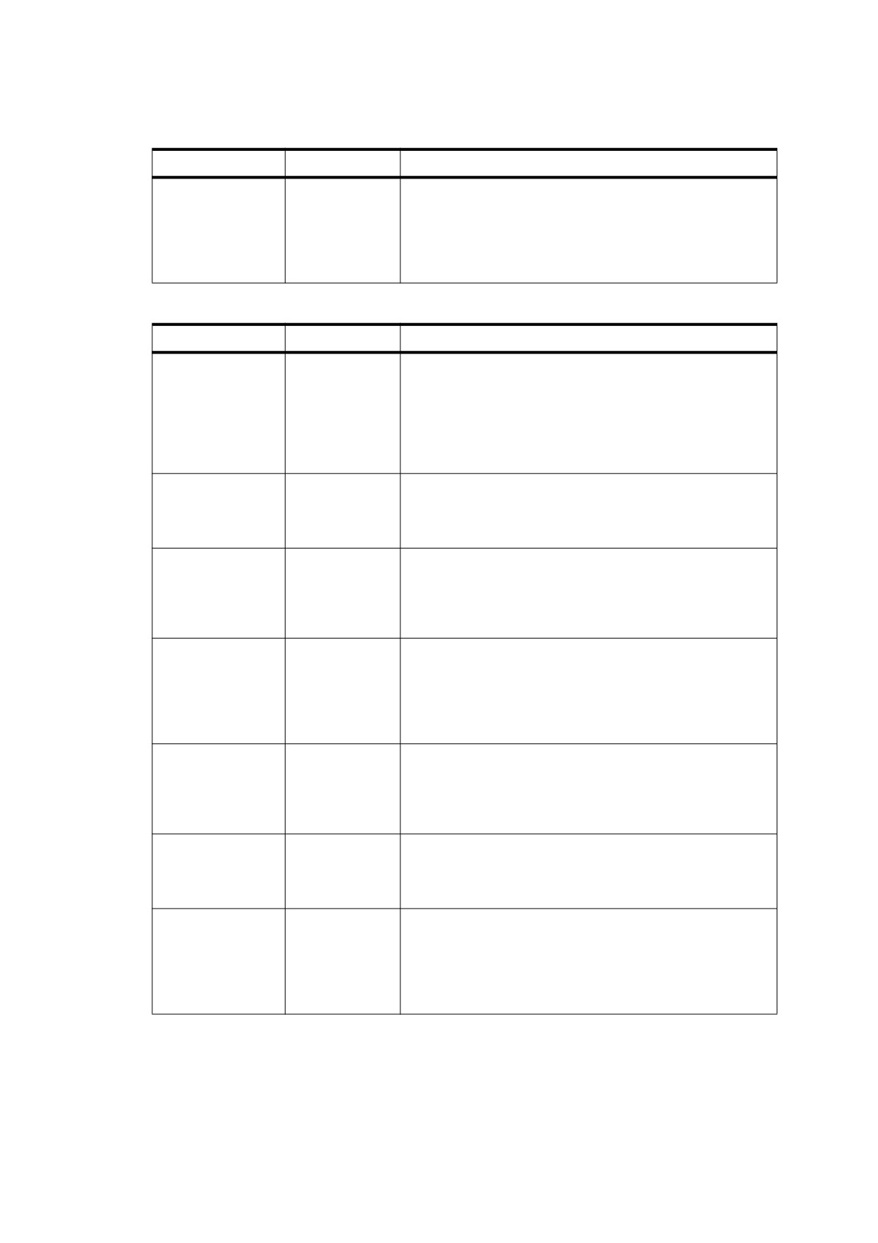
Table 52 - Device-Independent Graphics State Parameters (continued)

Parameter

Type

Value

alpha source

boolean

(PDF 1.4) A flag specifying whether the current soft mask and

alpha constant parameters shall be interpreted as shape

values (true) or opacity values (false). This flag also governs

the interpretation of the SMask entry, if any, in an image

dictionary

(see

8.9.5, "Image Dictionaries"). Initial value:

false.

Table 53 - Device-Dependent Graphics State Parameters

Parameter

Type

Value

overprint

boolean

(PDF 1.2) A flag specifying (on output devices that support

the overprint control feature) whether painting in one set of

colorants should cause the corresponding areas of other

colorants to be erased (false) or left unchanged (true); see

8.6.7, "Overprint Control". In PDF 1.3, there are two separate

overprint parameters: one for stroking and one for all other

painting operations. Initial value: false.

overprint mode

number

(PDF 1.3) A code specifying whether a colour component

value of 0 in a DeviceCMYK colour space should erase that

component (0) or leave it unchanged (1) when overprinting

(see 8.6.7, "Overprint Control"). Initial value: 0.

black generation

function

(PDF 1.2) A function that calculates the level of the black

or name

colour component to use when converting RGB colours to

CMYK

(see

10.3.4, "Conversion from DeviceRGB to

DeviceCMYK"). Initial value: a conforming reader shall

initialize this to a suitable device dependent value.

undercolor removal

function

(PDF 1.2) A function that calculates the reduction in the

or name

levels of the cyan, magenta, and yellow colour components to

compensate for the amount of black added by black

generation

(see

10.3.4, "Conversion from DeviceRGB to

DeviceCMYK"). Initial value: a conforming reader shall

initialize this to a suitable device dependent value.

transfer

function,

(PDF 1.2) A function that adjusts device gray or colour

array, or name

component levels to compensate for nonlinear response in a

particular output device

(see

10.4,

“Transfer Functions“).

Initial value: a conforming reader shall initialize this to a

suitable device dependent value.

halftone

dictionary,

(PDF 1.2) A halftone screen for gray and colour rendering,

stream, or name

specified as a halftone dictionary or stream

(see

10.5,

"Halftones"). Initial value: a conforming reader shall initialize

this to a suitable device dependent value.

flatness

number

The precision with which curves shall be rendered on the

output device (see 10.6.2, "Flatness Tolerance"). The value

of this parameter (positive number) gives the maximum error

tolerance, measured in output device pixels; smaller numbers

give smoother curves at the expense of more computation

and memory use. Initial value: 1.0.

123

Table 53 - Device-Dependent Graphics State Parameters (continued)

Parameter

Type

Value

smoothness

number

(PDF 1.3) The precision with which colour gradients are to be

rendered on the output device (see 10.6.3, "Smoothness

Tolerance"). The value of this parameter (0 to 1.0) gives the

maximum error tolerance, expressed as a fraction of the

range of each colour component; smaller numbers give

smoother colour transitions at the expense of more

computation and memory use. Initial value: a conforming

reader shall initialize this to a suitable device dependent

value.

NOTE 1

Some graphics state parameters are set with specific PDF operators, some are set by including a particular

entry in a graphics state parameter dictionary, and some can be specified either way.

EXAMPLE 2

The current line width can be set either with the w operator or (in PDF 1.3) with the LW entry in a graphics

state parameter dictionary, whereas the current colour is set only with specific operators, and the current

halftone is set only with a graphics state parameter dictionary.

In general, a conforming reader, when interpreting the operators that set graphics state parameters, shall

simply store them unchanged for later use when interpreting the painting operators.However, some parameters

have special properties or call for behaviour that a conforming reader shall handle:

•

Most parameters shall be of the correct type or have values that fall within a certain range.

•

Parameters that are numeric values, such as the current colour, line width, and miter limit, shall be forced

into valid range, if necessary. However, they shall not be adjusted to reflect capabilities of the raster output

device, such as resolution or number of distinguishable colours. Painting operators perform such

adjustments, but the adjusted values shall not be stored back into the graphics state.

•

Paths shall be internal objects that shall not be directly represented in PDF.

NOTE 2

As indicated in Table 52 and Table 53, some of the parameters—color space, color, and overprint—have two

values, one used for stroking (of paths and text objects) and one for all other painting operations. The two

parameter values can be set independently, allowing for operations such as combined filling and stroking of the

same path with different colours. Except where noted, a term such as current colour should be interpreted to

refer to whichever colour parameter applies to the operation being performed. When necessary, the individual

colour parameters are distinguished explicitly as the stroking colour and the nonstroking colour.

8.4.2

Graphics State Stack

A PDF document typically contains many graphical elements that are independent of each other and nested to

multiple levels. The graphics state stack allows these elements to make local changes to the graphics state

without disturbing the graphics state of the surrounding environment. The stack is a LIFO (last in, first out) data

structure in which the contents of the graphics state may be saved and later restored using the following

operators:

•

The q operator shall push a copy of the entire graphics state onto the stack.

•

The Q operator shall restore the entire graphics state to its former value by popping it from the stack.

NOTE

These operators can be used to encapsulate a graphical element so that it can modify parameters of the

graphics state and later restore them to their previous values.

Occurrences of the q and Q operators shall be balanced within a given content stream (or within the sequence

of streams specified in a page dictionary’s Contents array).

124

8.4.3

Details of Graphics State Parameters

8.4.3.1

General

This sub-clause gives details of several of the device-independent graphics state parameters listed in Table 52.

8.4.3.2

Line Width

The line width parameter specifies the thickness of the line used to stroke a path. It shall be a non-negative

number expressed in user space units; stroking a path shall entail painting all points whose perpendicular

distance from the path in user space is less than or equal to half the line width. The effect produced in device

space depends on the current transformation matrix (CTM) in effect at the time the path is stroked. If the CTM

specifies scaling by different factors in the horizontal and vertical dimensions, the thickness of stroked lines in

device space shall vary according to their orientation. The actual line width achieved can differ from the

requested width by as much as 2 device pixels, depending on the positions of lines with respect to the pixel

grid. Automatic stroke adjustment may be used to ensure uniform line width; see 10.6.5, "Automatic Stroke

Adjustment".

A line width of 0 shall denote the thinnest line that can be rendered at device resolution: 1 device pixel wide.

However, some devices cannot reproduce 1-pixel lines, and on high-resolution devices, they are nearly

invisible. Since the results of rendering such zero-width lines are device-dependent, they should not be used.

8.4.3.3

Line Cap Style

The line cap style shall specify the shape that shall be used at the ends of open subpaths (and dashes, if any)

when they are stroked. Table 54 shows the possible values.

Table 54 - Line Cap Styles

Style

Appearance

Description

0

Butt cap. The stroke shall be squared off at the endpoint

of the path.

There shall be no projection beyond the end of the path.

1

Round cap. A semicircular arc with a diameter equal to the line width

shall be drawn around the endpoint and shall be filled in.

2

Projecting square cap. The stroke shall continue beyond the endpoint

of the path for a distance equal to half the line width and shall be

squared off.

8.4.3.4

Line Join Style

The line join style shall specify the shape to be used at the corners of paths that are stroked. Table 55 shows

the possible values. Join styles shall be significant only at points where consecutive segments of a path

connect at an angle; segments that meet or intersect fortuitously shall receive no special treatment.

Table 55 - Line Join Styles

Style

Appearance

Description

0

Miter join. The outer edges of the strokes for the two segments shall be

extended until they meet at an angle, as in a picture frame. If the

segments meet at too sharp an angle (as defined by the miter limit

parameter—see 8.4.3.5, "Miter Limit"), a bevel join shall be used

instead.

125

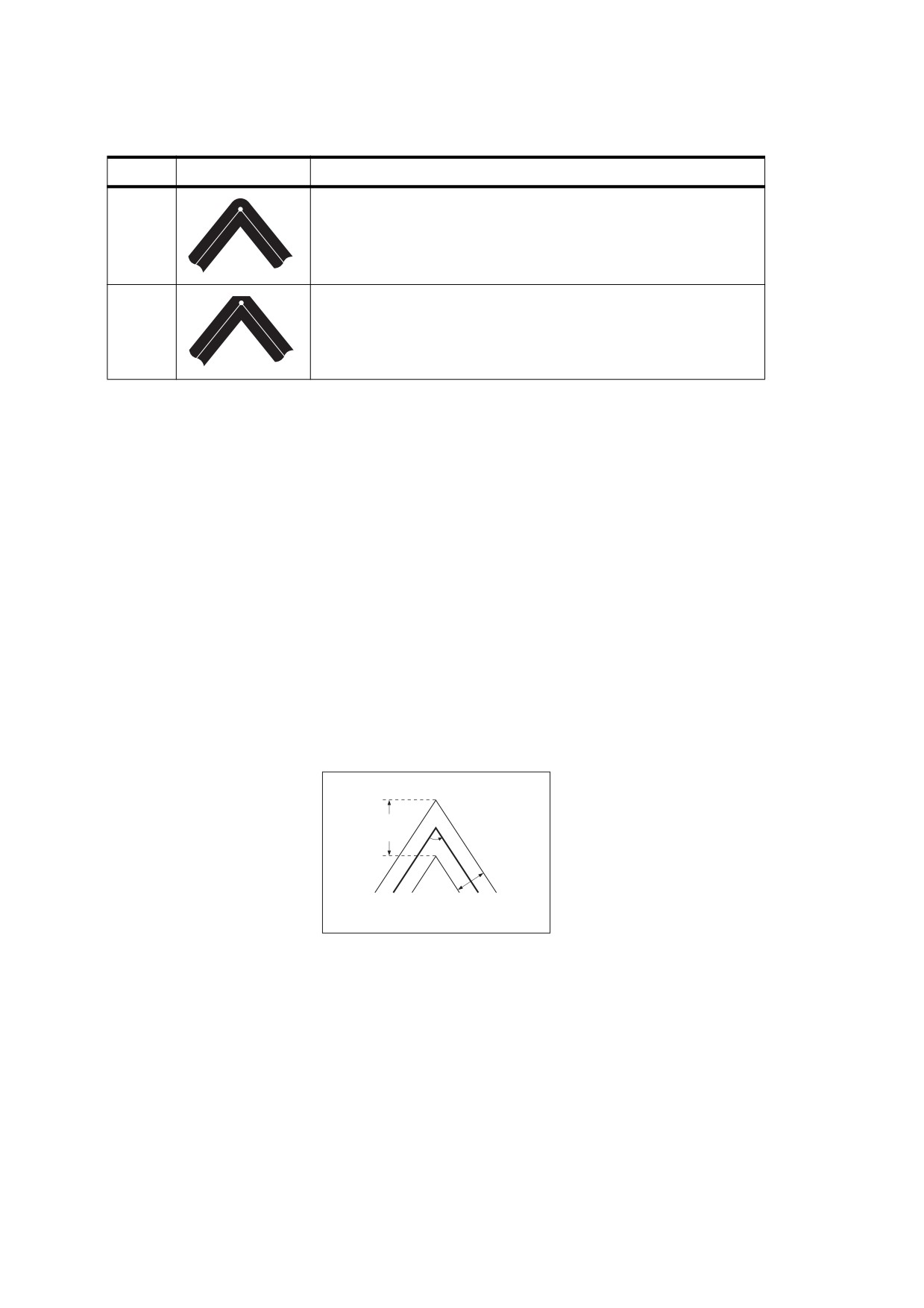
Table 55 - Line Join Styles (continued)

Style

Appearance

Description

1

Round join. An arc of a circle with a diameter equal to the line width

shall be drawn around the

point where the two segments meet,

connecting the outer edges of the strokes for the two segments. This

pieslice-shaped figure shall be filled in, producing a rounded corner.

2

Bevel join. The two segments shall be finished with butt caps (see

8.4.3.3, "Line Cap Style") and the resulting notch beyond the ends of

the segments shall be filled with a triangle.

NOTE

The definition of round join was changed in PDF 1.5. In rare cases, the implementation of the previous

specification could produce unexpected results.

8.4.3.5

Miter Limit

When two line segments meet at a sharp angle and mitered joins have been specified as the line join style, it is

possible for the miter to extend far beyond the thickness of the line stroking the path. The miter limit shall

impose a maximum on the ratio of the miter length to the line width (see Figure 15 in Annex L). When the limit

is exceeded, the join is converted from a miter to a bevel.

The ratio of miter length to line width is directly related to the angle j between the segments in user space by

the following formula:

miterLength

= ----------

--------

lineWidth

⎛

⎞

sin

--

⎝

2⎠

EXAMPLE

A miter limit of 1.414 converts miters to bevels for j less than 90 degrees, a limit of 2.0 converts them for j

less than 60 degrees, and a limit of 10.0 converts them for j less than approximately 11.5 degrees.

Miter

length

j

Line width

Figure 15 - Miter Length

8.4.3.6

Line Dash Pattern

The line dash pattern shall control the pattern of dashes and gaps used to stroke paths. It shall be specified by

a dash array and a dash phase. The dash array’s elements shall be numbers that specify the lengths of

alternating dashes and gaps; the numbers shall be nonnegative and not all zero. The dash phase shall specify

the distance into the dash pattern at which to start the dash. The elements of both the dash array and the dash

phase shall be expressed in user space units.

Before beginning to stroke a path, the dash array shall be cycled through, adding up the lengths of dashes and

gaps. When the accumulated length equals the value specified by the dash phase, stroking of the path shall

begin, and the dash array shall be used cyclically from that point onward. Table 56 shows examples of line

126

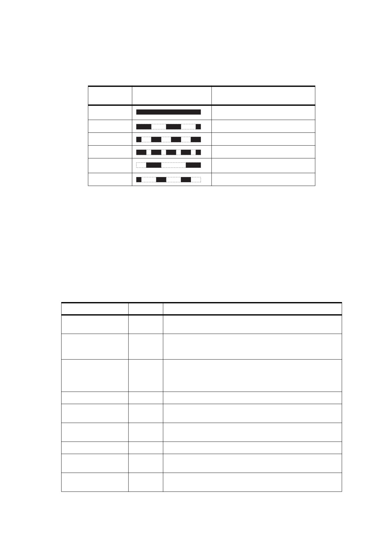
dash patterns. As can be seen from the table, an empty dash array and zero phase can be used to restore the

dash pattern to a solid line.

Table 56 - Examples of Line Dash Patterns

Dash Array

Appearance

Description

and Phase

[ ]

0

No dash; solid, unbroken lines

[3 ]

0

3 units on, 3 units off, …

[2 ]

1

1 on, 2 off, 2 on, 2 off, …

[2

1 ] 0

2 on, 1 off, 2 on, 1 off, …

[3

5 ] 6

2 off, 3 on, 5 off, 3 on, 5 off, …

[2

3 ] 11

1 on, 3 off, 2 on, 3 off, 2 on, …

Dashed lines shall wrap around curves and corners just as solid stroked lines do. The ends of each dash shall

be treated with the current line cap style, and corners within dashes shall be treated with the current line join

style. A stroking operation shall take no measures to coordinate the dash pattern with features of the path; it

simply shall dispense dashes and gaps along the path in the pattern defined by the dash array.

When a path consisting of several subpaths is stroked, each subpath shall be treated independently—that is,

the dash pattern shall be restarted and the dash phase shall be reapplied to it at the beginning of each subpath.

8.4.4

Graphics State Operators

Table 57 shows the operators that set the values of parameters in the graphics state. (See also the colour

operators listed in Table 74 and the text state operators in Table 105.)

Table 57 - Graphics State Operators

Operands

Operator

Description

—

q

Save the current graphics state on the graphics state stack (see

8.4.2, "Graphics State Stack").

—

Q

Restore the graphics state by removing the most recently saved

state from the stack and making it the current state (see 8.4.2,

"Graphics State Stack").

a b c d e f

cm

Modify the current transformation matrix (CTM) by concatenating

the specified matrix (see 8.3.2, "Coordinate Spaces"). Although the

operands specify a matrix, they shall be written as six separate

numbers, not as an array.

lineWidth

w

Set the line width in the graphics state (see 8.4.3.2, "Line Width").

lineCap

J

Set the line cap style in the graphics state (see 8.4.3.3, "Line Cap

Style").

lineJoin

j

Set the line join style in the graphics state (see 8.4.3.4, "Line Join

Style").

miterLimit

M

Set the miter limit in the graphics state (see 8.4.3.5, "Miter Limit").

dashArray dashPhase

d

Set the line dash pattern in the graphics state (see 8.4.3.6, "Line

Dash Pattern").

intent

ri

(PDF 1.1) Set the colour rendering intent in the graphics state (see

8.6.5.8, "Rendering Intents").

127

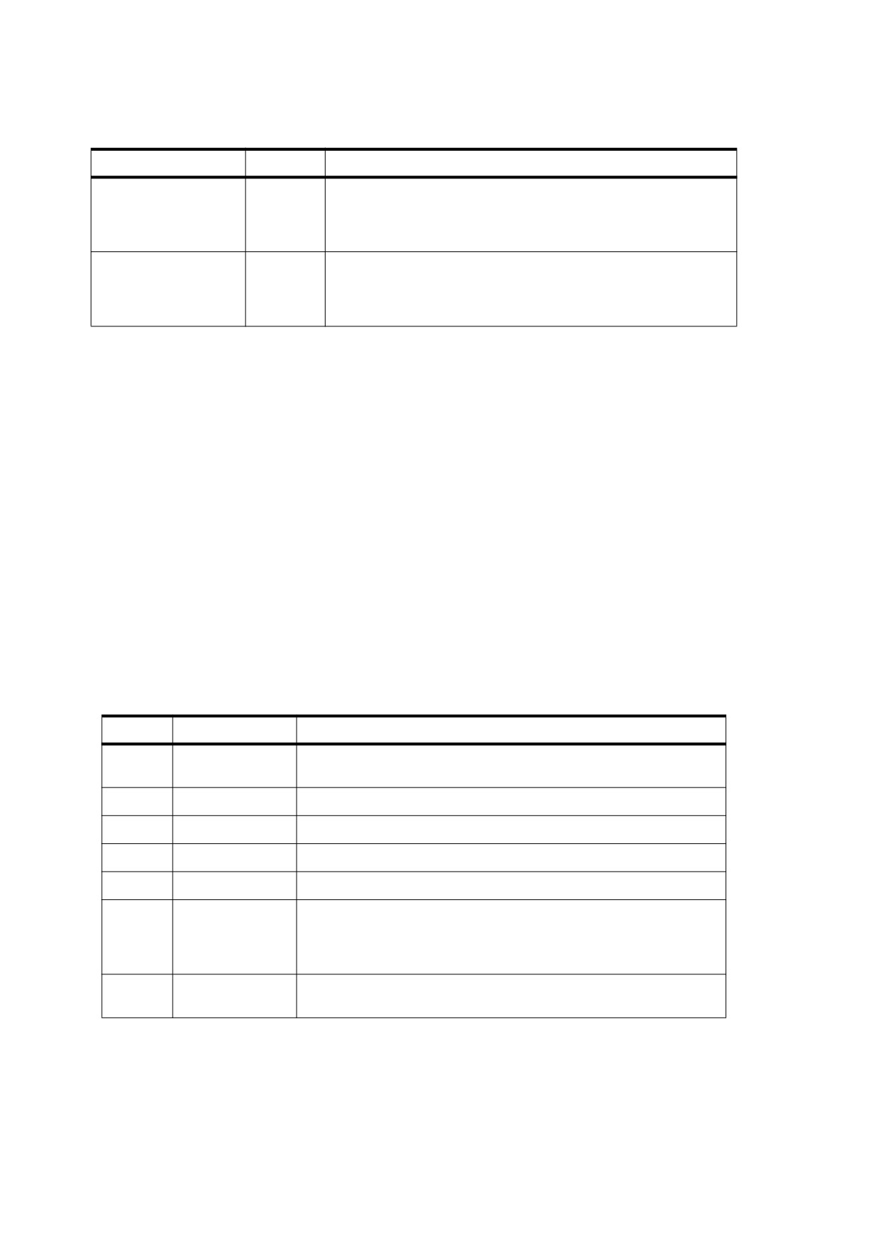
Table 57 - Graphics State Operators (continued)

Operands

Operator

Description

flatness

i

Set the flatness tolerance in the graphics state

(see

10.6.2,

"Flatness Tolerance"). flatness is a number in the range 0 to 100; a

value of

0 shall specify the output device’s default flatness

tolerance.

dictName

gs

(PDF 1.2) Set the specified parameters in the graphics state.

dictName shall be the name of a graphics state parameter

dictionary in the ExtGState subdictionary of the current resource

dictionary (see the next sub-clause).

8.4.5

Graphics State Parameter Dictionaries

While some parameters in the graphics state may be set with individual operators, as shown in Table 57, others

may not. The latter may only be set with the generic graphics state operator gs (PDF 1.2). The operand

supplied to this operator shall be the name of a graphics state parameter dictionary whose contents specify the

values of one or more graphics state parameters. This name shall be looked up in the ExtGState subdictionary

of the current resource dictionary.

The graphics state parameter dictionary is also used by type 2 patterns, which do not have a content stream in

which the graphics state operators could be invoked (see 8.7.4, "Shading Patterns").

Each entry in the parameter dictionary shall specify the value of an individual graphics state parameter, as

shown in Table 58. All entries need not be present for every invocation of the gs operator; the supplied

parameter dictionary may include any combination of parameter entries. The results of gs shall be cumulative;

parameter values established in previous invocations persist until explicitly overridden.

NOTE

Note that some parameters appear in both Table 57 and Table 58; these parameters can be set either with

individual graphics state operators or with gs. It is expected that any future extensions to the graphics state will

be implemented by adding new entries to the graphics state parameter dictionary rather than by introducing

new graphics state operators.

Table 58 - Entries in a Graphics State Parameter Dictionary

Key

Type

Description

Type

name

(Optional) The type of PDF object that this dictionary describes; shall

be ExtGState for a graphics state parameter dictionary.

LW

number

(Optional; PDF 1.3) The line width (see 8.4.3.2, "Line Width").

LC

integer

(Optional; PDF 1.3) The line cap style (see 8.4.3.3, "Line Cap Style").

LJ

integer

(Optional; PDF 1.3) The line join style (see 8.4.3.4, "Line Join Style").

ML

number

(Optional; PDF 1.3) The miter limit (see 8.4.3.5, "Miter Limit").

D

array

(Optional; PDF 1.3) The line dash pattern, expressed as an array of

the form [ dashArray dashPhase ], where dashArray shall be itself an

array and dashPhase shall be an integer (see 8.4.3.6, "Line Dash

Pattern").

RI

name

(Optional; PDF 1.3) The name of the rendering intent (see 8.6.5.8,

"Rendering Intents").

128

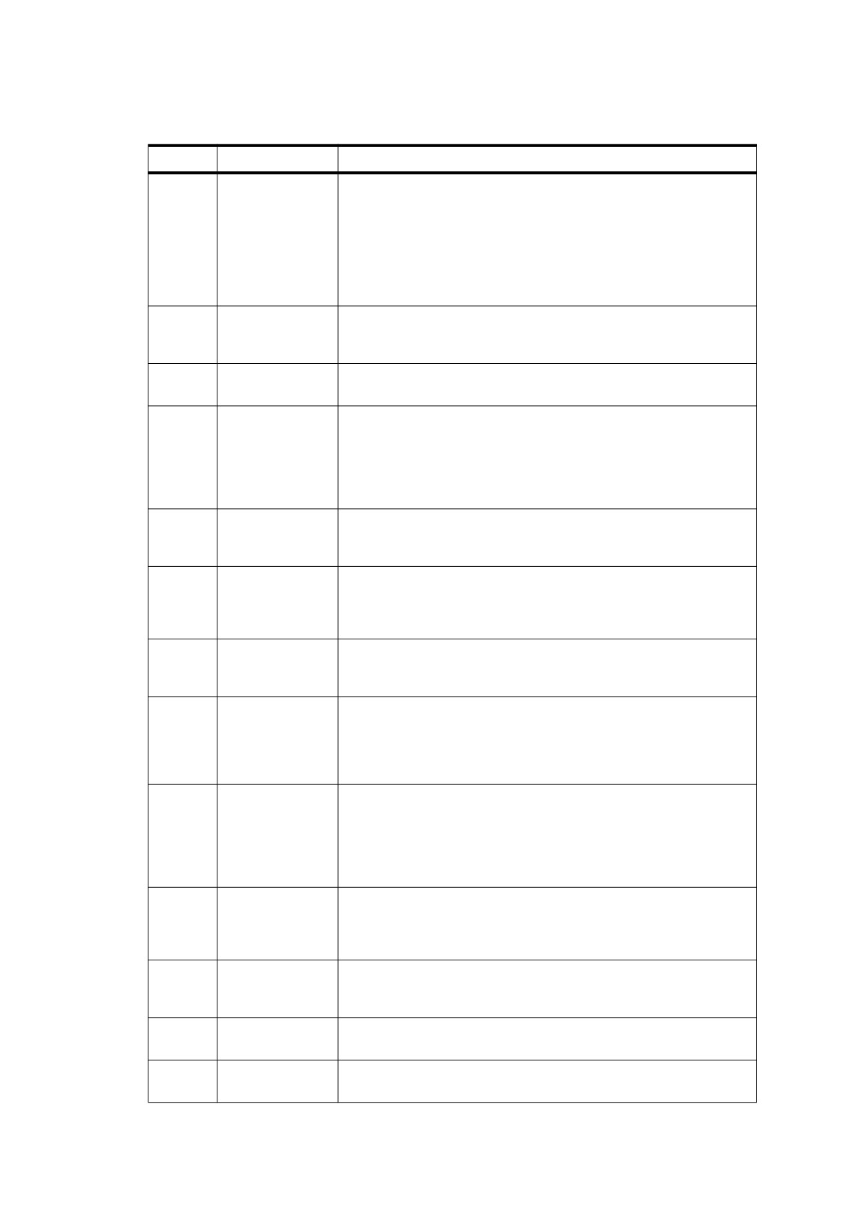
Table 58 - Entries in a Graphics State Parameter Dictionary (continued)

Key

Type

Description

OP

boolean

(Optional) A flag specifying whether to apply overprint (see 8.6.7,

"Overprint Control"). In PDF 1.2 and earlier, there is a single overprint

parameter that applies to all painting operations. Beginning with PDF

1.3, there shall be two separate overprint parameters: one for stroking

and one for all other painting operations. Specifying an OP entry shall

set both parameters unless there is also an op entry in the same

graphics state parameter dictionary, in which case the OP entry shall

set only the overprint parameter for stroking.

op

boolean

(Optional; PDF 1.3) A flag specifying whether to apply overprint (see

8.6.7, "Overprint Control") for painting operations other than stroking. If

this entry is absent, the OP entry, if any, shall also set this parameter.

OPM

integer

(Optional; PDF 1.3) The overprint mode

(see

8.6.7, "Overprint

Control").

Font

array

(Optional; PDF 1.3) An array of the form [ font size ], where font shall

be an indirect reference to a font dictionary and size shall be a number

expressed in text space units. These two objects correspond to the

operands of the Tf operator (see 9.3, "Text State Parameters and

Operators"); however, the first operand shall be an indirect object

reference instead of a resource name.

BG

function

(Optional) The black-generation function, which maps the interval

[0.0

1.0 ] to the interval

[0.0

1.0 ]

(see

10.3.4, "Conversion from

DeviceRGB to DeviceCMYK").

BG2

function or name

(Optional; PDF 1.3) Same as BG except that the value may also be

the name Default, denoting the black-generation function that was in

effect at the start of the page. If both BG and BG2 are present in the

same graphics state parameter dictionary, BG2 shall take precedence.

UCR

function

(Optional) The undercolor-removal function, which maps the interval

[0.0

1.0 ] to the interval

[−1.0

1.0 ]

(see 10.3.4, "Conversion from

DeviceRGB to DeviceCMYK").

UCR2

function or name

(Optional; PDF 1.3) Same as UCR except that the value may also be

the name Default, denoting the undercolor-removal function that was

in effect at the start of the page. If both UCR and UCR2 are present in

the same graphics state parameter dictionary, UCR2 shall take

precedence.

TR

function, array, or

(Optional) The transfer function, which maps the interval [ 0.0 1.0 ] to

name

the interval [ 0.0

1.0 ] (see 10.4, "Transfer Functions"). The value shall

be either a single function (which applies to all process colorants) or

an array of four functions

(which apply to the process colorants

individually). The name Identity may be used to represent the identity

function.

TR2

function, array, or

(Optional; PDF 1.3) Same as TR except that the value may also be the

name

name Default, denoting the transfer function that was in effect at the

start of the page. If both TR and TR2 are present in the same graphics

state parameter dictionary, TR2 shall take precedence.

HT

dictionary,

(Optional) The halftone dictionary or stream (see 10.5, "Halftones") or

stream, or name

the name Default, denoting the halftone that was in effect at the start of

the page.

FL

number

(Optional; PDF 1.3) The flatness tolerance

(see

10.6.2, "Flatness

Tolerance").

SM

number

(Optional; PDF 1.3) The smoothness tolerance

(see

10.6.3,

"Smoothness Tolerance").

129

Table 58 - Entries in a Graphics State Parameter Dictionary (continued)

Key

Type

Description

SA

boolean

(Optional) A flag specifying whether to apply automatic stroke

adjustment (see 10.6.5, "Automatic Stroke Adjustment").

BM

name or array

(Optional; PDF 1.4) The current blend mode to be used in the

transparent imaging model (see 11.3.5, "Blend Mode" and 11.6.3,

"Specifying Blending Colour Space and Blend Mode").

SMask

dictionary

or

(Optional; PDF 1.4) The current soft mask, specifying the mask shape

name

or mask opacity values that shall be used in the transparent imaging

model (see 11.3.7.2, "Source Shape and Opacity" and 11.6.4.3, "Mask

Shape and Opacity").

Although the current soft mask is sometimes referred to as a “soft clip,”

altering it with the gs operator completely replaces the old value with

the new one, rather than intersecting the two as is done with the

current clipping path parameter (see 8.5.4, "Clipping Path Operators").

CA

number

(Optional; PDF 1.4) The current stroking alpha constant, specifying the

constant shape or constant opacity value that shall be used for

stroking operations in the transparent imaging model (see 11.3.7.2,

"Source Shape and Opacity" and 11.6.4.4, "Constant Shape and

Opacity").

ca

number

(Optional; PDF 1.4) Same as CA, but for nonstroking operations.

AIS

boolean

(Optional; PDF 1.4) The alpha source flag

(“alpha is shape”),

specifying whether the current soft mask and alpha constant shall be

interpreted as shape values (true) or opacity values (false).

TK

boolean

(Optional; PDF 1.4) The text knockout flag, shall determine the

behaviour of overlapping glyphs within a text object in the transparent

imaging model (see 9.3.8, "Text Knockout").

EXAMPLE

The following shows two graphics state parameter dictionaries. In the first, automatic stroke adjustment is

turned on, and the dictionary includes a transfer function that inverts its value, f (x) = 1 - x. In the second,

overprint is turned off, and the dictionary includes a parabolic transfer function, f (x) = (2x - 1) ², with a

sample of 21 values. The domain of the transfer function, [ 0.0 1.0 ], is mapped to [ 0 20 ], and the range

of the sample values, [ 0 255 ], is mapped to the range of the transfer function, [ 0.0 1.0 ].

10 0 obj

% Page object

<< /Type /Page

/Parent 5 0 R

/Resources 20 0 R

/Contents 40 0 R

>>

endobj

20 0 obj

% Resource dictionary for page

<<

/ProcSet [ /PDF /Text ]

/Font << /F1 25 0 R >>

/ExtGState << /GS1 30 0 R

/GS2 35 0 R

>>

>>

endobj

30 0 obj

% First graphics state parameter dictionary

<<

/Type /ExtGState

/SA true

/TR 31 0 R

>>

endobj

130

As discussed in 8.2, "Graphics Objects", a path object is defined by a sequence of operators to construct the

path, followed by one or more operators to paint the path or to use it as a clipping boundary. PDF path

operators fall into three categories:

•

Path construction operators (8.5.2, "Path Construction Operators") define the geometry of a path. A path is

constructed by sequentially applying one or more of these operators.

•

Path-painting operators (8.5.3, "Path-Painting Operators") end a path object, usually causing the object to

be painted on the current page in any of a variety of ways.

•

Clipping path operators (8.5.4, "Clipping Path Operators"), invoked immediately before a path-painting

operator, cause the path object also to be used for clipping of subsequent graphics objects.

8.5.2

Path Construction Operators

8.5.2.1

General

A page description shall begin with an empty path and shall build up its definition by invoking one or more path

construction operators to add segments to it. The path construction operators may be invoked in any sequence,

but the first one invoked shall be m or re to begin a new subpath. The path definition may conclude with the

application of a path-painting operator such as S, f, or b (see 8.5.3, "Path-Painting Operators"); this operator

may optionally be preceded by one of the clipping path operators W or W* (8.5.4, "Clipping Path Operators").

NOTE

Note that the path construction operators do not place any marks on the page; only the painting operators do

that. A path definition is not complete until a path-painting operator has been applied to it.

The path currently under construction is called the current path. In PDF (unlike PostScript), the current path is

not part of the graphics state and is not saved and restored along with the other graphics state parameters.

PDF paths shall be strictly internal objects with no explicit representation. After the current path has been

painted, it shall become no longer defined; there is then no current path until a new one is begun with the m or

re operator.

The trailing endpoint of the segment most recently added to the current path is referred to as the current point.

If the current path is empty, the current point shall be undefined. Most operators that add a segment to the

current path start at the current point; if the current point is undefined, an error shall be generated.

Table 59 shows the path construction operators. All operands shall be numbers denoting coordinates in user

space.

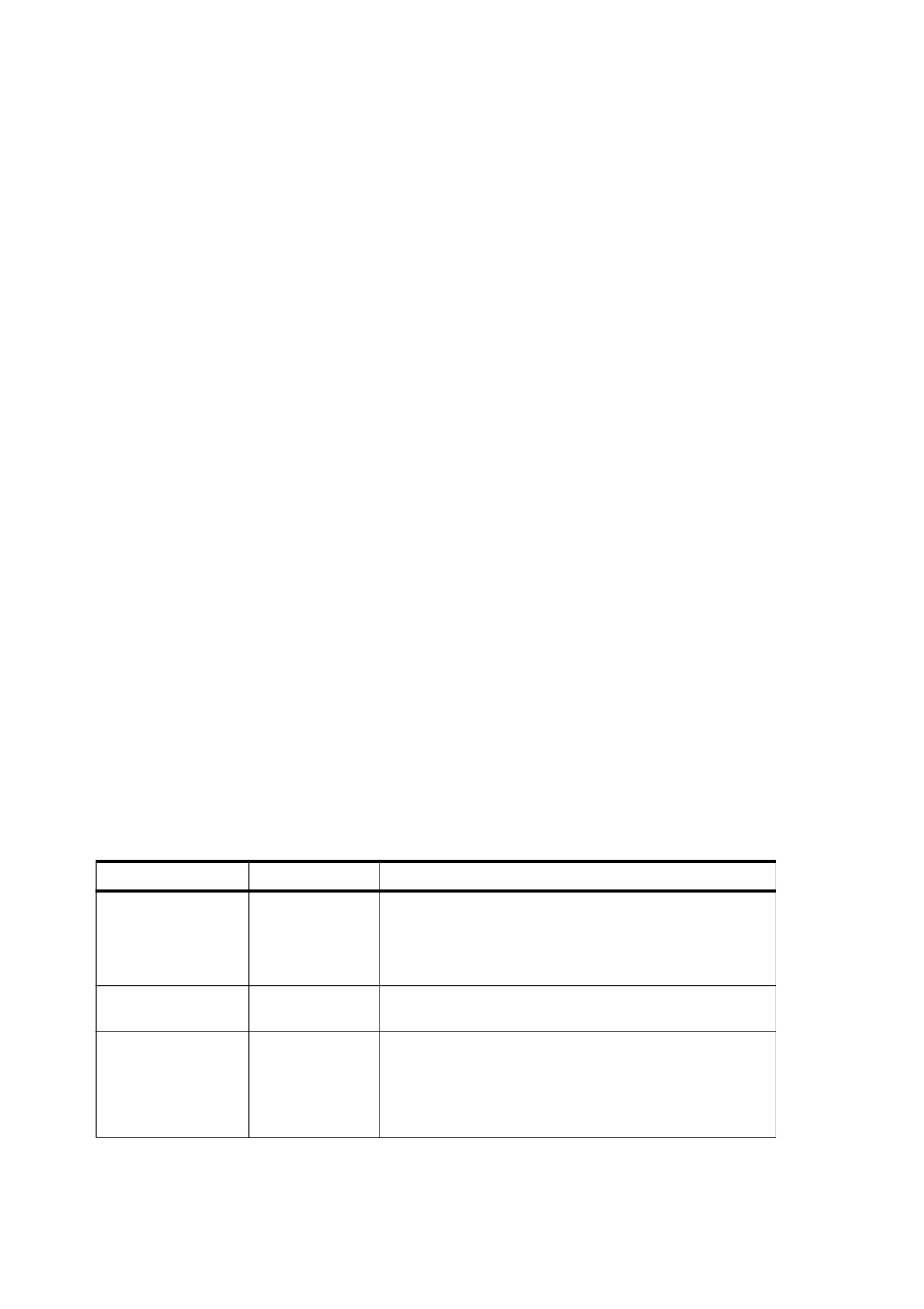
Table 59 - Path Construction Operators

Operands

Operator

Description

x y

m

Begin a new subpath by moving the current point to

coordinates (x, y), omitting any connecting line segment. If

the previous path construction operator in the current path

was also m, the new m overrides it; no vestige of the

previous m operation remains in the path.

x y

l (lowercase L)

Append a straight line segment from the current point to the

point (x, y). The new current point shall be (x, y).

x₁ y₁ x₂ y₂ x₃ y₃

c

Append a cubic Bézier curve to the current path. The curve

shall extend from the current point to the point (x₃ , y₃ ), using

(x₁ , y₁ ) and (x₂ , y₂ ) as the Bézier control points (see 8.5.2.2,

"Cubic Bézier Curves"). The new current point shall be

(x₃ , y₃ ).

132

Table 59 - Path Construction Operators (continued)

Operands

Operator

Description

x₂ y₂ x₃ y₃

v

Append a cubic Bézier curve to the current path. The curve

shall extend from the current point to the point (x₃ , y₃ ), using

the current point and (x₂ , y₂ ) as the Bézier control points (see

8.5.2.2, "Cubic Bézier Curves"). The new current point shall

be (x₃ , y₃ ).

x₁ y₁ x₃ y₃

y

Append a cubic Bézier curve to the current path. The curve

shall extend from the current point to the point (x₃ , y₃ ), using

(x₁ , y₁ ) and (x₃ , y₃ ) as the Bézier control points (see 8.5.2.2,

"Cubic Bézier Curves"). The new current point shall be

(x₃ , y₃ ).

—

h

Close the current subpath by appending a straight line

segment from the current point to the starting point of the

subpath. If the current subpath is already closed, h shall do

nothing.

This operator terminates the current subpath. Appending

another segment to the current path shall begin a new

subpath, even if the new segment begins at the endpoint

reached by the h operation.

x y width height

re

Append a rectangle to the current path as a complete

subpath, with lower-left corner (x, y) and dimensions width

and height in user space. The operation

x y width height re

is equivalent to

x y m

( x + width ) y l

( x + width )

( y + height ) l

x ( y + height ) l

h

8.5.2.2

Cubic Bézier Curves

Curved path segments shall be specified as cubic Bézier curves. Such curves shall be defined by four points:

the two endpoints (the current point P₀ and the final point P₃ ) and two control points P₁ and P₂ . Given the

coordinates of the four points, the curve shall be generated by varying the parameter t from 0.0 to 1.0 in the

following equation:

R (t)

=

(1-t)³P₀

+

3t(1-t)²P₁

+

3t²(1 - t)P₂

+

t³P₃

When t = 0.0, the value of the function R (t) coincides with the current point P₀ ; when t = 1.0, R (t) coincides with

the final point P₃ . Intermediate values of t generate intermediate points along the curve. The curve does not, in

general, pass through the two control points P₁ and P₂ .

NOTE 1

Cubic Bézier curves have two useful properties:

The curve can be very quickly split into smaller pieces for rapid rendering.

The curve is contained within the convex hull of the four points defining the curve, most easily visualized as the

polygon obtained by stretching a rubber band around the outside of the four points. This property allows rapid

testing of whether the curve lies completely outside the visible region, and hence does not have to be

rendered.

NOTE 2

The Bibliography lists several books that describe cubic Bézier curves in more depth.

133

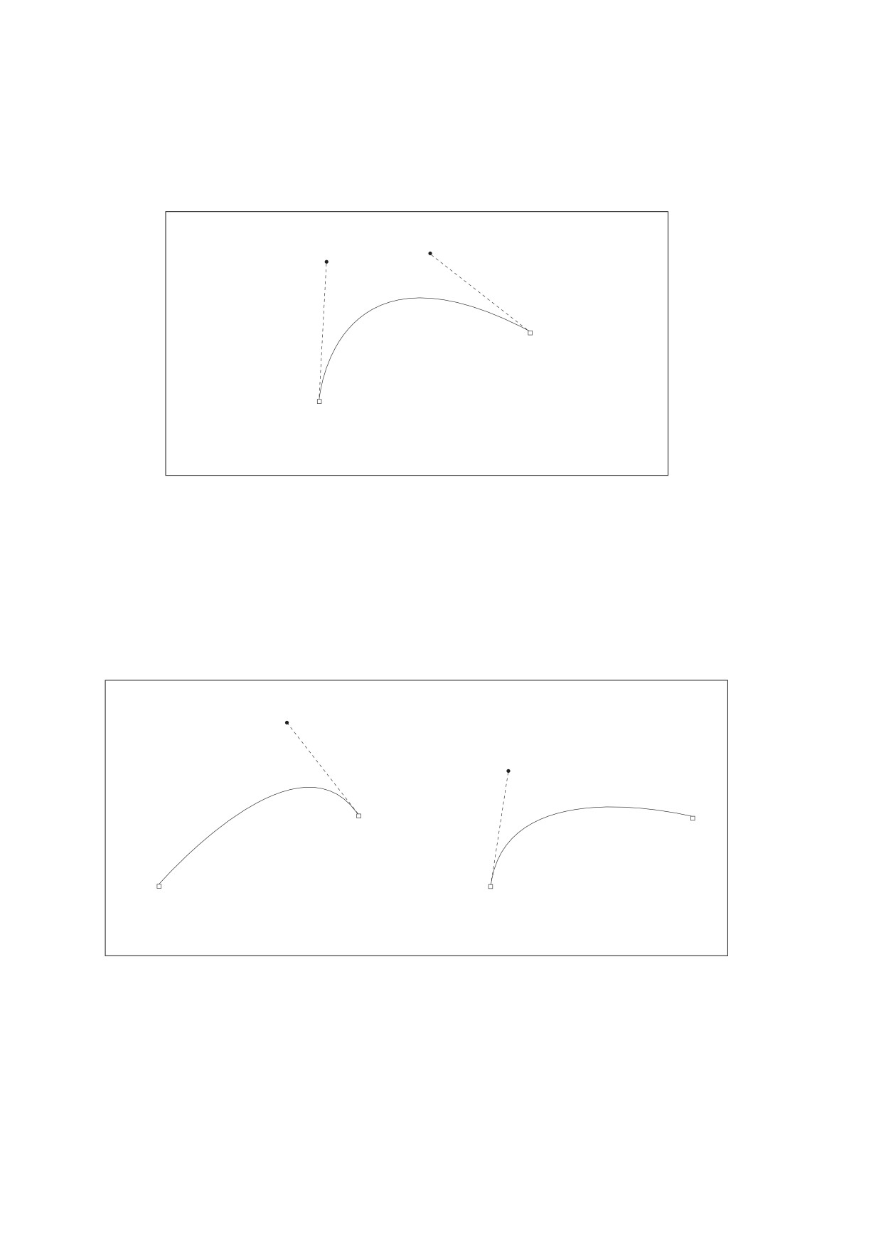
The most general PDF operator for constructing curved path segments is the c operator, which specifies the

coordinates of points P₁ , P₂ , and P₃ explicitly, as shown in Figure 16 in Annex L. (The starting point, P₀ , is

defined implicitly by the current point.)

P₂ (x₂

, y₂

)

P₁ (x₁, y₁

)

P₃ (x₃

, y₃

)

P₀ (current point)

x₁ y₁ x₂ y₂ x₃ y₃ c

Figure 16 - Cubic Bézier Curve Generated by the c Operator

Two more operators, v and y, each specify one of the two control points implicitly (see Figure 17 in Annex L). In

both of these cases, one control point and the final point of the curve shall be supplied as operands; the other

control point shall be implied:

•

For the v operator, the first control point shall coincide with initial point of the curve.

•

For the y operator, the second control point shall coincide with final point of the curve.

(x₂

,

y₂

)

(x₁

,

y₁

)

(x₃

,

y₃

)

(x₃

,

y₃

)

Current point

Current point

x₂ y₂ x₃ y₃ v

x₁ y₁ x₃ y₃ y

Figure 17 - Cubic Bézier Curves Generated by the v and y Operators

8.5.3

Path-Painting Operators

8.5.3.1

General

The path-painting operators end a path object, causing it to be painted on the current page in the manner that

the operator specifies. The principal path-painting operators shall be S (for stroking) and f (for filling). Variants

134

of these operators combine stroking and filling in a single operation or apply different rules for determining the

area to be filled. Table 60 lists all the path-painting operators.

Table 60 - Path-Painting Operators

Operands

Operator

Description

—

S

Stroke the path.

—

s

Close and stroke the path. This operator shall have the same effect as the

sequence h S.

—

f

Fill the path, using the nonzero winding number rule to determine the region

to fill

(see 8.5.3.3.2, "Nonzero Winding Number Rule"). Any subpaths that

are open shall be implicitly closed before being filled.

—

F

Equivalent to f; included only for compatibility. Although PDF reader

applications shall be able to accept this operator, PDF writer applications

should use f instead.

—

f*

Fill the path, using the even-odd rule to determine the region to fill (see

8.5.3.3.3, "Even-Odd Rule").

—

B

Fill and then stroke the path, using the nonzero winding number rule to

determine the region to fill. This operator shall produce the same result as

constructing two identical path objects, painting the first with f and the

second with S.

NOTE

The filling and stroking portions of the operation consult

different values of several graphics state parameters, such as

the current colour. See also 11.7.4.4, "Special Path-Painting

Considerations".

—

B*

Fill and then stroke the path, using the even-odd rule to determine the region

to fill. This operator shall produce the same result as B, except that the path

is filled as if with f* instead of f. See also 11.7.4.4, "Special Path-Painting

Considerations".

—

b

Close, fill, and then stroke the path, using the nonzero winding number rule

to determine the region to fill. This operator shall have the same effect as the

sequence h B. See also 11.7.4.4, "Special Path-Painting Considerations".

—

b*

Close, fill, and then stroke the path, using the even-odd rule to determine the

region to fill. This operator shall have the same effect as the sequence h B*.

See also 11.7.4.4, "Special Path-Painting Considerations".

—

n

End the path object without filling or stroking it. This operator shall be a path-

painting no-op, used primarily for the side effect of changing the current

clipping path (see 8.5.4, "Clipping Path Operators").

8.5.3.2

Stroking

The S operator shall paint a line along the current path. The stroked line shall follow each straight or curved

segment in the path, centred on the segment with sides parallel to it. Each of the path’s subpaths shall be

treated separately.

The results of the S operator shall depend on the current settings of various parameters in the graphics state

(see 8.4, "Graphics State", for further information on these parameters):

•

The width of the stroked line shall be determined by the current line width parameter (8.4.3.2, "Line

Width").

•

The colour or pattern of the line shall be determined by the current colour and colour space for stroking

operations.

135

The method just described does not specify what to do if a path segment coincides with or is tangent to the

chosen ray. Since the direction of the ray is arbitrary, the rule simply chooses a ray that does not encounter

such problem intersections.

For simple convex paths, the nonzero winding number rule defines the inside and outside as one would

intuitively expect. The more interesting cases are those involving complex or self-intersecting paths like the

ones shown in Figure 18 in Annex L. For a path consisting of a five-pointed star, drawn with five connected

straight line segments intersecting each other, the rule considers the inside to be the entire area enclosed by

the star, including the pentagon in the centre. For a path composed of two concentric circles, the areas

enclosed by both circles are considered to be inside, provided that both are drawn in the same direction. If the

circles are drawn in opposite directions, only the doughnut shape between them is inside, according to the rule;

the doughnut hole is outside.

Figure 18 - Nonzero Winding Number Rule

8.5.3.3.3 Even-Odd Rule

An alternative to the nonzero winding number rule is the even-odd rule. This rule determines whether a point is

inside a path by drawing a ray from that point in any direction and simply counting the number of path segments

that cross the ray, regardless of direction. If this number is odd, the point is inside; if even, the point is outside.

This yields the same results as the nonzero winding number rule for paths with simple shapes, but produces

different results for more complex shapes.

Figure 19 shows the effects of applying the even-odd rule to complex paths. For the five-pointed star, the rule

considers the triangular points to be inside the path, but not the pentagon in the centre. For the two concentric

circles, only the doughnut shape between the two circles is considered inside, regardless of the directions in

which the circles are drawn.

Figure 19 - Even-Odd Rule

8.5.4

Clipping Path Operators

The graphics state shall contain a current clipping path that limits the regions of the page affected by painting

operators. The closed subpaths of this path shall define the area that can be painted. Marks falling inside this

area shall be applied to the page; those falling outside it shall not be. Sub-clause 8.5.3.3, "Filling" discusses

precisely what shall be considered to be inside a path.

137

In the context of the transparent imaging model (PDF 1.4), the current clipping path constrains an object’s

shape (see 11.2, "Overview of Transparency"). The effective shape is the intersection of the object’s intrinsic

shape with the clipping path; the source shape value shall be 0.0 outside this intersection. Similarly, the shape

of a transparency group (defined as the union of the shapes of its constituent objects) shall be influenced both

by the clipping path in effect when each of the objects is painted and by the one in effect at the time the group’s

results are painted onto its backdrop.

The initial clipping path shall include the entire page. A clipping path operator (W or W*, shown in Table 61)

may appear after the last path construction operator and before the path-painting operator that terminates a

path object. Although the clipping path operator appears before the painting operator, it shall not alter the

clipping path at the point where it appears. Rather, it shall modify the effect of the succeeding painting operator.

After the path has been painted, the clipping path in the graphics state shall be set to the intersection of the

current clipping path and the newly constructed path.

Table 61 - Clipping Path Operators

Operands

Operator

Description

—

W

Modify the current clipping path by intersecting it with the current path, using

the nonzero winding number rule to determine which regions lie inside the

clipping path.

—

W*

Modify the current clipping path by intersecting it with the current path, using

the even-odd rule to determine which regions lie inside the clipping path.

NOTE 1

In addition to path objects, text objects may also be used for clipping; see 9.3.6, "Text Rendering Mode".

The n operator (see Table 60) is a no-op path-painting operator; it shall cause no marks to be placed on the

page, but can be used with a clipping path operator to establish a new clipping path. That is, after a path has

been constructed, the sequence W n shall intersect that path with the current clipping path and shall establish a

new clipping path.

NOTE 2

There is no way to enlarge the current clipping path or to set a new clipping path without reference to the

current one. However, since the clipping path is part of the graphics state, its effect can be localized to specific

graphics objects by enclosing the modification of the clipping path and the painting of those objects between a

pair of q and Q operators (see 8.4.2, "Graphics State Stack"). Execution of the Q operator causes the clipping

path to revert to the value that was saved by the q operator before the clipping path was modified.

8.6

Colour Spaces

8.6.1

General

PDF includes facilities for specifying the colours of graphics objects to be painted on the current page. The

colour facilities are divided into two parts:

•

Colour specification. A conforming writer may specify abstract colours in a device-independent way.

Colours may be described in any of a variety of colour systems, or colour spaces. Some colour spaces are

related to device colour representation (grayscale, RGB, CMYK), others to human visual perception (CIE-

based). Certain special features are also modelled as colour spaces: patterns, colour mapping,

separations, and high-fidelity and multitone colour.

•

Colour rendering. A conforming reader shall reproduce colours on the raster output device by a multiple-

step process that includes some combination of colour conversion, gamma correction, halftoning, and

scan conversion. Some aspects of this process use information that is specified in PDF. However, unlike

the facilities for colour specification, the colour-rendering facilities are device-dependent and should not be

included in a page description.

Figure 20 and Figure 21 illustrate the division between PDF’s (device-independent) colour specification and

(device-dependent) colour-rendering facilities. This sub-clause describes the colour specification features,

covering everything that PDF documents need to specify colours. The facilities for controlling colour rendering

138

are described in clause 10, "Rendering"; a conforming writer should use these facilities only to configure or

calibrate an output device or to achieve special device-dependent effects.

8.6.2

Colour Values

As described in 8.5.3, "Path-Painting Operators", marks placed on the page by operators such as f and S shall

have a colour that is determined by the current colour parameter of the graphics state. A colour value consists

of one or more colour components, which are usually numbers. A gray level shall be specified by a single

number ranging from 0.0 (black) to 1.0 (white). Full colour values may be specified in any of several ways; a

common method uses three numeric values to specify red, green, and blue components.

Colour values shall be interpreted according to the current colour space, another parameter of the graphics

state. A PDF content stream first selects a colour space by invoking the CS operator (for the stroking colour) or

the cs operator (for the nonstroking colour). It then selects colour values within that colour space with the SC

operator (stroking) or the sc operator (nonstroking). There are also convenience operators—G, g, RG, rg, K,

and k—that select both a colour space and a colour value within it in a single step. Table 74 lists all the colour-

setting operators.

Sampled images (see 8.9, "Images") specify the colour values of individual samples with respect to a colour

space designated by the image object itself. While these values are independent of the current colour space

and colour parameters in the graphics state, all later stages of colour processing shall treat them in exactly the

same way as colour values specified with the SC or sc operator.

8.6.3

Colour Space Families

Colour spaces are classified into colour space families. Spaces within a family share the same general

characteristics; they shall be distinguished by parameter values supplied at the time the space is specified. The

families fall into three broad categories:

•

Device colour spaces directly specify colours or shades of gray that the output device shall produce. They

provide a variety of colour specification methods, including grayscale, RGB (red-green-blue), and CMYK

(cyan-magenta-yellow-black), corresponding to the colour space families DeviceGray, DeviceRGB, and

DeviceCMYK. Since each of these families consists of just a single colour space with no parameters, they

may be referred to as the DeviceGray, DeviceRGB, and DeviceCMYK colour spaces.

•

CIE-based colour spaces shall be based on an international standard for colour specification created by

the Commission Internationale de l’Éclairage (International Commission on Illumination). These spaces

specify colours in a way that is independent of the characteristics of any particular output device. Colour

space families in this category include CalGray, CalRGB, Lab, and ICCBased. Individual colour spaces

within these families shall be specified by means of dictionaries containing the parameter values needed to

define the space.

•

Special colour spaces add features or properties to an underlying colour space. They include facilities for

patterns, colour mapping, separations, and high-fidelity and multitone colour. The corresponding colour

space families are Pattern, Indexed, Separation, and DeviceN. Individual colour spaces within these

families shall be specified by means of additional parameters.

Table 62 summarizes the colour space families in PDF.

Table 62 - Colour Space Families

Device

CIE-based

Special

DeviceGray (PDF 1.1)

CalGray (PDF 1.1)

Indexed (PDF 1.1)

DeviceRGB (PDF 1.1)

CalRGB (PDF 1.1)

Pattern (PDF 1.2)

DeviceCMYK (PDF 1.1)

Lab (PDF 1.1)

Separation (PDF 1.2)

ICCBased (PDF 1.3)

DeviceN (PDF 1.3)

139

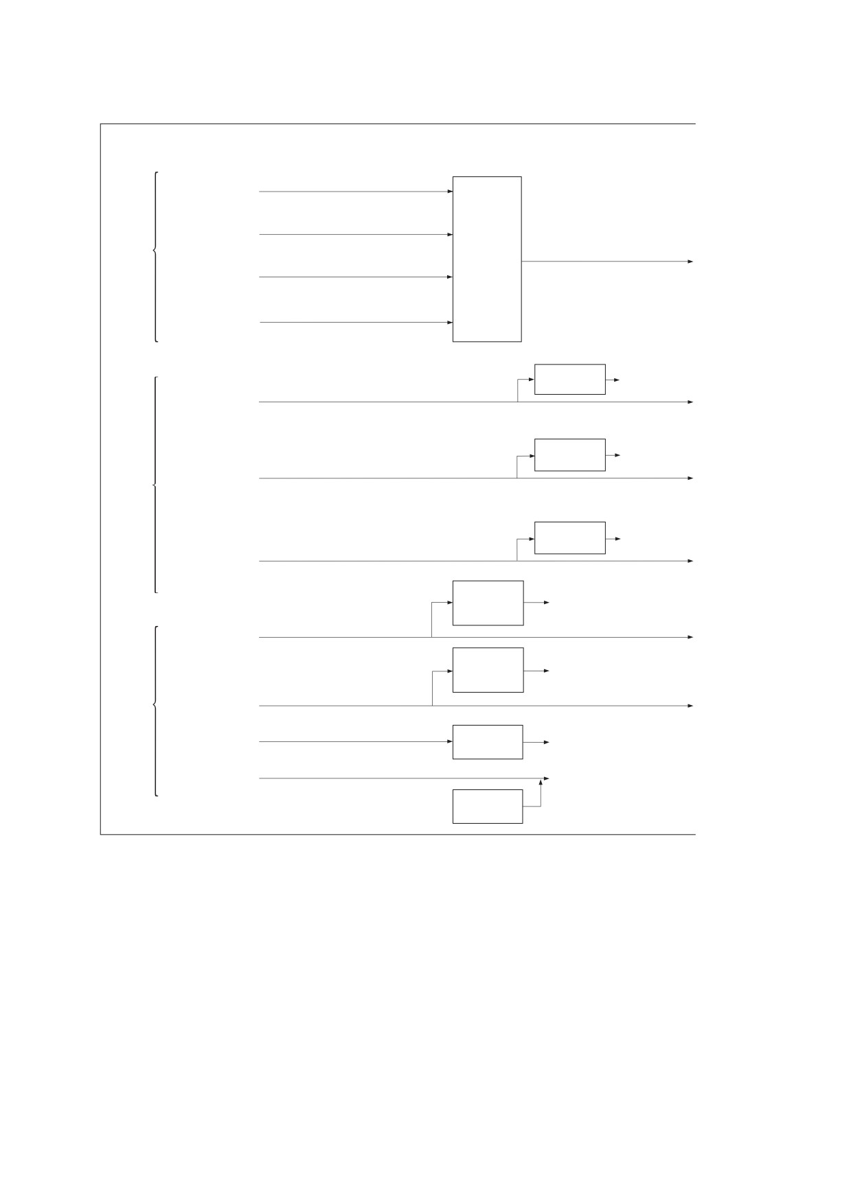
Sources of

Color spaces

color values

Color values

A, B, C

CalRGB

sc, SC, sh,

BI, Do (image XObject)

CIE-

A

CalGray

based

sc, SC, sh,

Conversion

BI, Do (image XObject)

to internal

X, Y, Z

color

A, B, C

X, Y, Z

spaces

Lab

values

sc, SC, sh,

BI, Do (image XObject)

n

components

ICCBased

scn, SCN, sh,

BI, Do (image XObject)

Another

DefaultRGB

(3-component)

R, G, B

color space

DeviceRGB

rg, RG, sc, SC, sh,

BI, Do (image XObject)

Another

DefaultCMYK

(4-component)

Device

C, M, Y, K

color space

DeviceCMYK

color

k, K, sc, SC, sh,

spaces

BI, Do (image XObject)

Another

DefaultGray

(1-component)

gray

color space

DeviceGray

g, G, sc, SC, sh,

BI, Do (image XObject)

Alternative

Another

color

color space

transform

tint

Separation

scn, SCN, sh,

BI, Do (image XObject)

Alternative

Another

color

color space

n

transform

Special

components

color

DeviceN

scn, SCN, sh,

spaces

BI, Do (image XObject)

index

Table

Another

Indexed

lookup

color space

sc, SC, sh,

BI, Do (image XObject)

pattern

Another

Pattern

color space

scn, SCN

Pattern

dictionary

Figure 20 - Colour Specification

140

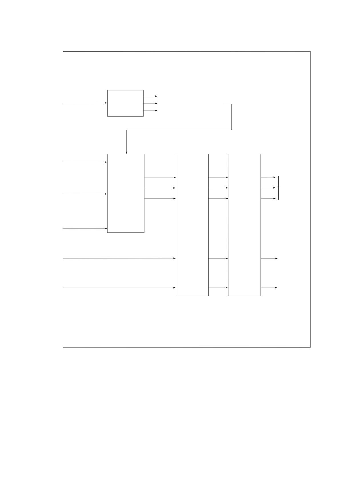
Conversion

R, G, B

Device color values

X, Y, Z

from CIE-based

(depending on

C, M, Y, K

to device

results of

color space

gray

conversion)

(not specified by PDF)

R, G, B

Component(s)

of device’s

process

color model

Conversion

from input

Device’s

device color

process

C, M, Y, K

space to

colorant(s)

device’s

process color

model

Transfer

Halftones

functions

gray

(per

(per

component)

component)

UCR, BG

Any single

tint

device

colorant

n

components

Any n device

colorants

TR, HT

HT

Figure 21 - Colour Rendering

A colour space shall be defined by an array object whose first element is a name object identifying the colour

space family. The remaining array elements, if any, are parameters that further characterize the colour space;

their number and types vary according to the particular family. For families that do not require parameters, the

colour space may be specified simply by the family name itself instead of an array.

A colour space shall be specified in one of two ways:

•

Within a content stream, the CS or cs operator establishes the current colour space parameter in the

graphics state. The operand shall always be name object, which either identifies one of the colour spaces

that need no additional parameters (DeviceGray, DeviceRGB, DeviceCMYK, or some cases of Pattern)

or shall be used as a key in the ColorSpace subdictionary of the current resource dictionary (see 7.8.3,

141

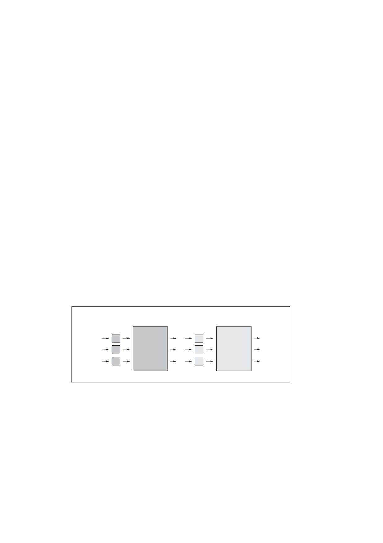
8.6.5

CIE-Based Colour Spaces

8.6.5.1

General

Calibrated colour in PDF shall be defined in terms of an international standard used in the graphic arts,

television, and printing industries. CIE-based colour spaces enable a page description to specify colour values

in a way that is related to human visual perception. The goal is for the same colour specification to produce

consistent results on different output devices, within the limitations of each device; Figure L.2 in Annex L

illustrates the kind of variation in colour reproduction that can result from the use of uncalibrated colour on

different devices. PDF 1.1 supports three CIE-based colour space families, named CalGray, CalRGB, and

Lab; PDF 1.3 added a fourth, named ICCBased.

NOTE 1

In PDF 1.1, a colour space family named CalCMYK was partially defined, with the expectation that its definition

would be completed in a future version. However, this feature has been deprecated. PDF 1.3 and later

versions support calibrated four-component colour spaces by means of ICC profiles (see 8.6.5.5, "ICCBased

Colour Spaces"). A conforming reader should ignore CalCMYK colour space attributes and render colours

specified in this family as if they had been specified using DeviceCMYK.

NOTE 2

The details of the CIE colourimetric system and the theory on which it is based are beyond the scope of this

specification; see the Bibliography for sources of further information. The semantics of CIE-based colour

spaces are defined in terms of the relationship between the space’s components and the tristimulus values X,

Y, and Z of the CIE 1931 XYZ space. The CalRGB and Lab colour spaces (PDF 1.1) are special cases of

three-component CIE-based colour spaces, known as CIE-based ABC colour spaces. These spaces are

defined in terms of a two-stage, nonlinear transformation of the CIE 1931 XYZ space. The formulation of such

colour spaces models a simple zone theory of colour vision, consisting of a nonlinear trichromatic first stage

combined with a nonlinear opponent-colour second stage. This formulation allows colours to be digitized with

minimum loss of fidelity, an important consideration in sampled images.

Colour values in a CIE-based ABC colour space shall have three components, arbitrarily named A, B, and C.

The first stage shall transform these components by first forcing their values to a specified range, then applying

decoding functions, and then multiplying the results by a

3-by-3 matrix, producing three intermediate

components arbitrarily named L, M, and N. The second stage shall transform these intermediate components

in a similar fashion, producing the final X, Y, and Z components of the CIE 1931 XYZ space (see Figure 22).

Decode ABC

Decode LMN

A

L

X

Matrix ABC

Matrix LMN

B

M

Y

C

N

Z

Figure 22 - Component Transformations in a CIE-based ABC Colour Space

Colour spaces in the CIE-based families shall be defined by an array

[name dictionary ]

where name is the name of the family and dictionary is a dictionary containing parameters that further

characterize the space. The entries in this dictionary have specific interpretations that depend on the colour

space; some entries are required and some are optional. See the sub-clauses on specific colour space families

for details.

Setting the current stroking or nonstroking colour space to any CIE-based colour space shall initialize all

components of the corresponding current colour to 0.0 (unless the range of valid values for a given component

does not include 0.0, in which case the nearest valid value shall be substituted.)

144

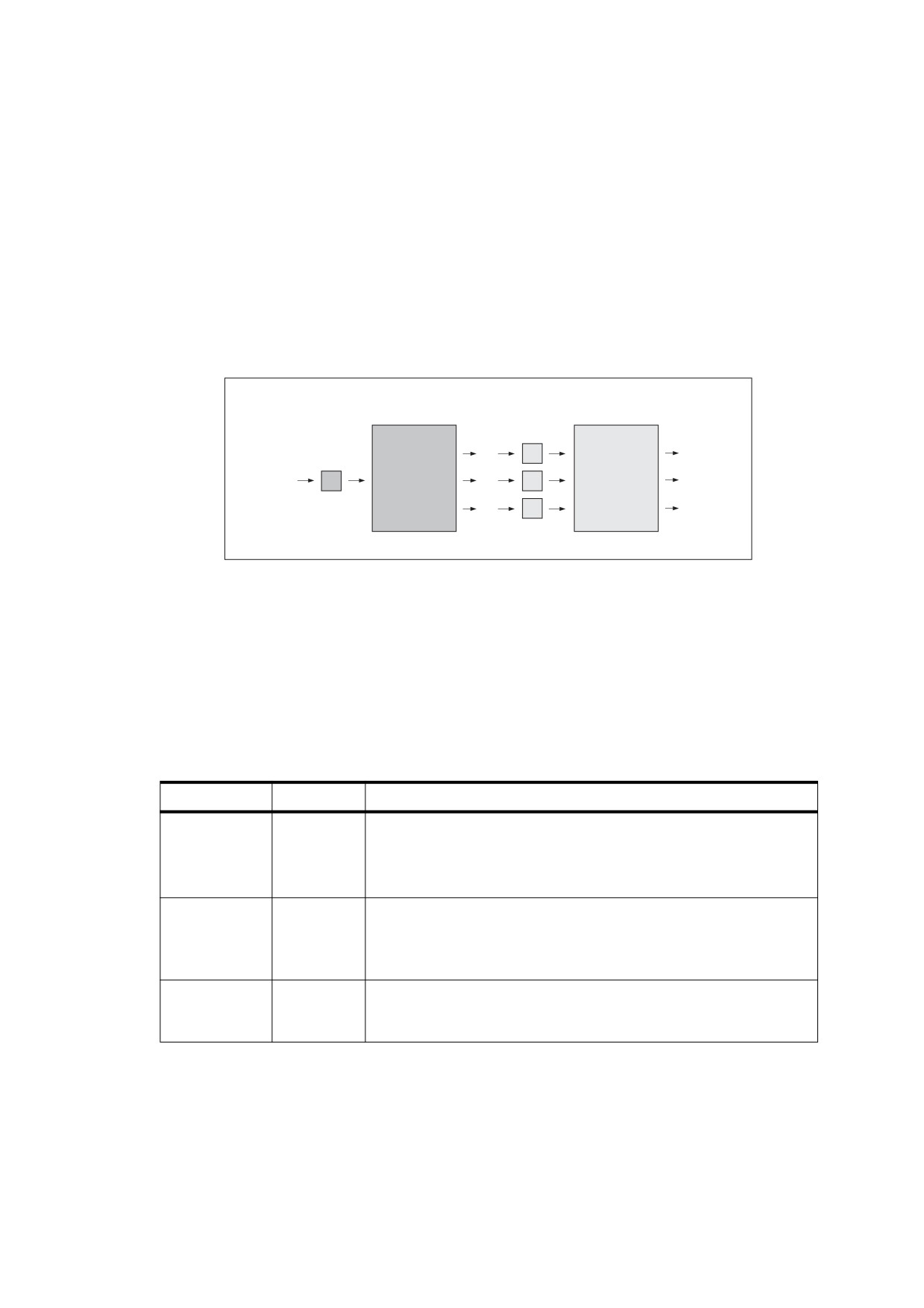
NOTE 3

The model and terminology used here—CIE-based ABC (above) and CIE-based A (below)—are derived from

the PostScript language, which supports these colour space families in their full generality. PDF supports

specific useful cases of CIE-based ABC and CIE-based A spaces; most others can be represented as

ICCBased spaces.

8.6.5.2

CalGray Colour Spaces

A CalGray colour space (PDF 1.1) is a special case of a single-component CIE-based colour space, known as

a CIE-based A colour space. This type of space is the one-dimensional (and usually achromatic) analog of CIE-

based ABC spaces. Colour values in a CIE-based A space shall have a single component, arbitrarily named A.

Figure 23 illustrates the transformations of the A component to X, Y, and Z components of the CIE 1931 XYZ

space.

Decode A

Decode LMN

L

X

A

Matrix A

M

Matrix LMN

Y

N

Z

Figure 23 - Component Transformations in a CIE-based A Colour Space

A CalGray colour space shall be a CIE-based A colour space with only one transformation stage instead of

two. In this type of space, A represents the gray component of a calibrated gray space. This component shall

be in the range 0.0 to 1.0. The decoding function (denoted by “Decode A” in Figure 23) is a gamma function

whose coefficient shall be specified by the Gamma entry in the colour space dictionary (see Table 63). The

transformation matrix denoted by “Matrix A” in the figure is derived from the dictionary’s WhitePoint entry, as

described below. Since there is no second transformation stage, “Decode LMN” and “Matrix LMN” shall be

implicitly taken to be identity transformations.

Table 63 - Entries in a CalGray Colour Space Dictionary

Key

Type

Value

WhitePoint

array

(Required) An array of three numbers [ X_W Y_W Z_W ] specifying the

tristimulus value, in the CIE 1931 XYZ space, of the diffuse white point;

see 8.6.5.3, "CalRGB Colour Spaces", for further discussion. The

numbers X_W and Z_W shall be positive, and Y_W shall be equal to 1.0.

BlackPoint

array

(Optional) An array of three numbers

[X_B Y_B Z_B ] specifying the

tristimulus value, in the CIE 1931 XYZ space, of the diffuse black point;

see 8.6.5.3, "CalRGB Colour Spaces", for further discussion. All three

of these numbers shall be non-negative. Default value: [ 0.0 0.0 0.0 ].

Gamma

number

(Optional) A number G defining the gamma for the gray

(A)

component. G shall be positive and is generally greater than or equal

to 1. Default value: 1.

The transformation defined by the Gamma and WhitePoint entries is

X = L = X_W × A^G

Y = M = Y_W × A^G

Z = N = Z_W × A^G

145

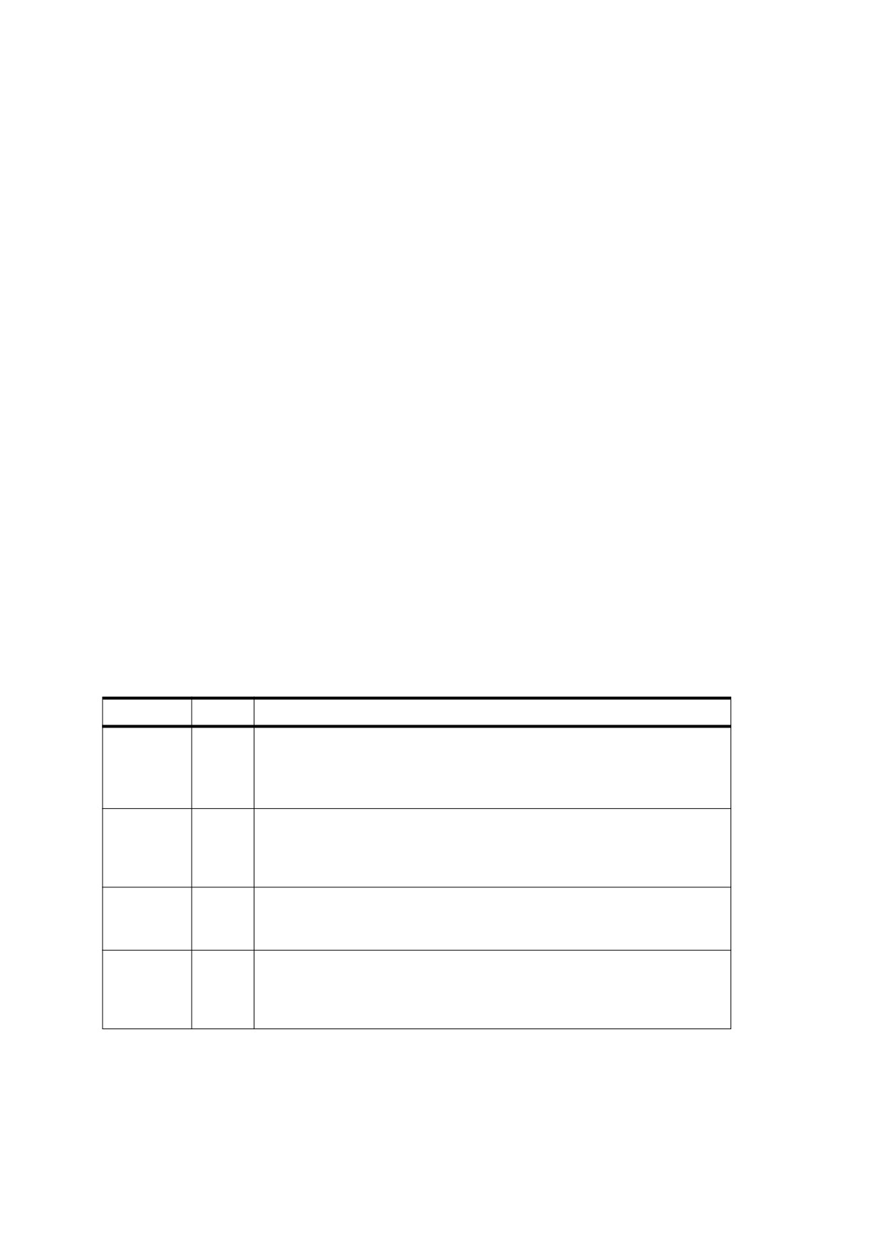
In other words, the A component shall be first decoded by the gamma function, and the result shall be

multiplied by the components of the white point to obtain the L, M, and N components of the intermediate

representation. Since there is no second stage, the L, M, and N components shall also be the X, Y, and Z

components of the final representation.

EXAMPLE 1

The examples in this sub-clause illustrate interesting and useful special cases of CalGray spaces. This

example establishes a space consisting of the Y dimension of the CIE 1931 XYZ space with the CCIR XA/

11-recommended D65 white point.

[ /CalGray

<< /WhitePoint [ 0.9505 1.0000 1.0890 ] >>

]

EXAMPLE 2

This example establishes a calibrated gray space with the CCIR XA/11-recommended D65 white point

and opto-electronic transfer function.

[ /CalGray

<<

/WhitePoint [ 0.9505 1.0000 1.0890 ]

/Gamma 2.222

>>

]

8.6.5.3

CalRGB Colour Spaces

A CalRGB colour space is a CIE-based ABC colour space with only one transformation stage instead of two. In

this type of space, A, B, and C represent calibrated red, green, and blue colour values. These three colour

components shall be in the range 0.0 to 1.0; component values falling outside that range shall be adjusted to

the nearest valid value without error indication. The decoding functions (denoted by “Decode ABC” in Figure

22) are gamma functions whose coefficients shall be specified by the Gamma entry in the colour space

dictionary (see Table 64). The transformation matrix denoted by “Matrix ABC” in Figure 22 shall be defined by

the dictionary’s Matrix entry. Since there is no second transformation stage, “Decode LMN” and “Matrix LMN”

shall be implicitly taken to be identity transformations.

Table 64 - Entries in a CalRGB Colour Space Dictionary

Key

Type

Value

WhitePoint

array

(Required) An array of three numbers [ X_W Y_W Z_W ] specifying the tristimulus

value, in the CIE 1931 XYZ space, of the diffuse white point; see below for

further discussion. The numbers X_W and Z_W shall be positive, and Y_W shall be

equal to 1.0.

BlackPoint

array

(Optional) An array of three numbers [ X_B Y_B Z_B] specifying the tristimulus

value, in the CIE 1931 XYZ space, of the diffuse black point; see below for

further discussion. All three of these numbers shall be non-negative. Default

value: [ 0.0

0.0 0.0 ].

Gamma

array

(Optional) An array of three numbers [ G_R G_G G_B ] specifying the gamma for

the red, green, and blue (A, B, and C) components of the colour space.

Default value: [ 1.0

1.0 1.0 ].

Matrix

array

(Optional) An array of nine numbers

[X_A Y_A Z_A X_B Y_B Z_B X_C Y_C Z_C]

specifying the linear interpretation of the decoded A, B, and C components of

the colour space with respect to the final XYZ representation. Default value:

the identity matrix [ 1

0 0 0 1 0 0 0 1 ].

The WhitePoint and BlackPoint entries in the colour space dictionary shall control the overall effect of the

CIE-based gamut mapping function described in sub-clause 10.2, "CIE-Based Colour to Device Colour".

Typically, the colours specified by WhitePoint and BlackPoint shall be mapped to the nearly lightest and

nearly darkest achromatic colours that the output device is capable of rendering in a way that preserves colour

appearance and visual contrast.

146

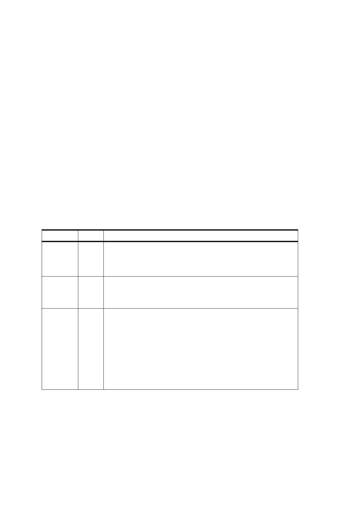
y_B

(

x_R – x_G

)× y_W

–

(

x_W – x_G

)× y_R

+

(

x_W x_R

)×y

Y_C

=

------

× ----------------------------------------------------------------------------------------------------------------------------------

B

z

x_B

⎛1

-

x_B

⎞

X_C = YC

× ------

Z_C = YC

×

⎜

---------------

- 1

⎟

y

y_B

B

⎝

⎠

X_W = X_A × R + X_B × G + X_C × B

Y_W = Y_A × R + Y_B × G + Y_C × B

Z_W = Z_A × R + Z_B × G + Z_C × B

8.6.5.4

Lab Colour Spaces

A Lab colour space is a CIE-based ABC colour space with two transformation stages (see Figure 22). In this

type of space, A, B, and C represent the L*, a*, and b* components of a CIE 1976 L*a*b* space. The range of

the first (L*) component shall be 0 to 100; the ranges of the second and third (a* and b*) components shall be

defined by the Range entry in the colour space dictionary (see Table 65).

Figure L.3 in Annex L illustrates the coordinates of a typical Lab colour space; Figure L.4 in Annex L compares

the gamuts (ranges of representable colours) for L*a*b*, RGB, and CMYK spaces.

Table 65 - Entries in a Lab Colour Space Dictionary

Key

Type

Value

WhitePoint

array

(Required) An array of three numbers [ X_W Y_W Z_W ] that shall specify the

tristimulus value, in the CIE 1931 XYZ space, of the diffuse white point; see

8.6.5.3, "CalRGB Colour Spaces" for further discussion. The numbers X_W and

Z_W shall be positive, and Y_W shall be 1.0.

BlackPoint

array

(Optional) An array of three numbers

[X_B Y_B Z_B ] that shall specify the

tristimulus value, in the CIE 1931 XYZ space, of the diffuse black point; see

8.6.5.3, "CalRGB Colour Spaces" for further discussion. All three of these

numbers shall be non-negative. Default value: [ 0.0 0.0 0.0 ].

Range

array

(Optional) An array of four numbers [ a_min a_max b_min b_max] that shall specify

the range of valid values for the a* and b* (B and C) components of the colour

space—that is,

a_min ≤ a* ≤ a_max

and

b_min ≤ b* ≤ b_max

Component values falling outside the specified range shall be adjusted to the

nearest valid value without error indication.

Default value: [−100 100 −100 100 ].

A Lab colour space shall not specify explicit decoding functions or matrix coefficients for either stage of the

transformation from L*a*b* space to XYZ space (denoted by “Decode ABC,” “Matrix ABC,” “Decode LMN,” and

“Matrix LMN” in Figure

22). Instead, these parameters shall have constant implicit values. The first

transformation stage shall be defined by the equations

148

L = L^*+16

+ --------

116

500

M = L^*+16

116

N = L*+16

- --------

116

200

The second transformation stage shall be

X = X_W × g(L)

Y = Y_W × g(M)

Z = Z_W × g(N)

where the function g (x) shall be defined as

-

g(x)

=

x³

if x

≥ ---

29

108

-

⎛

⎞

g(x)

=

×

x

- ---

otherwise

841

⎝

29⎠

EXAMPLE

The following defines the CIE 1976 L*a*b* space with the CCIR XA/11-recommended D65 white point.

The a* and b* components, although theoretically unbounded, are defined to lie in the useful range -128

to +127.

[ /Lab

<<

/WhitePoint [ 0.9505 1.0000 1.0890 ]

/Range [ -128 127 -128 127 ]

>>

]

8.6.5.5

ICCBased Colour Spaces

ICCBased colour spaces (PDF 1.3) shall be based on a cross-platform colour profile as defined by the

International Color Consortium (ICC) (see, “Bibliography“). Unlike the CalGray, CalRGB, and Lab colour

spaces, which are characterized by entries in the colour space dictionary, an ICCBased colour space shall be

characterized by a sequence of bytes in a standard format. Details of the profile format can be found in the ICC

specification (see, “Bibliography“).

An ICCBased colour space shall be an array:

[ /ICCBased stream ]

The stream shall contain the ICC profile. Besides the usual entries common to all streams (see Table 5), the

profile stream shall have the additional entries listed in Table 66.

Table 66 - Additional Entries Specific to an ICC Profile Stream Dictionary

Key

Type

Value

N

integer

(Required) The number of colour components in the colour space described

by the ICC profile data. This number shall match the number of components

actually in the ICC profile. N shall be 1, 3, or 4.

149

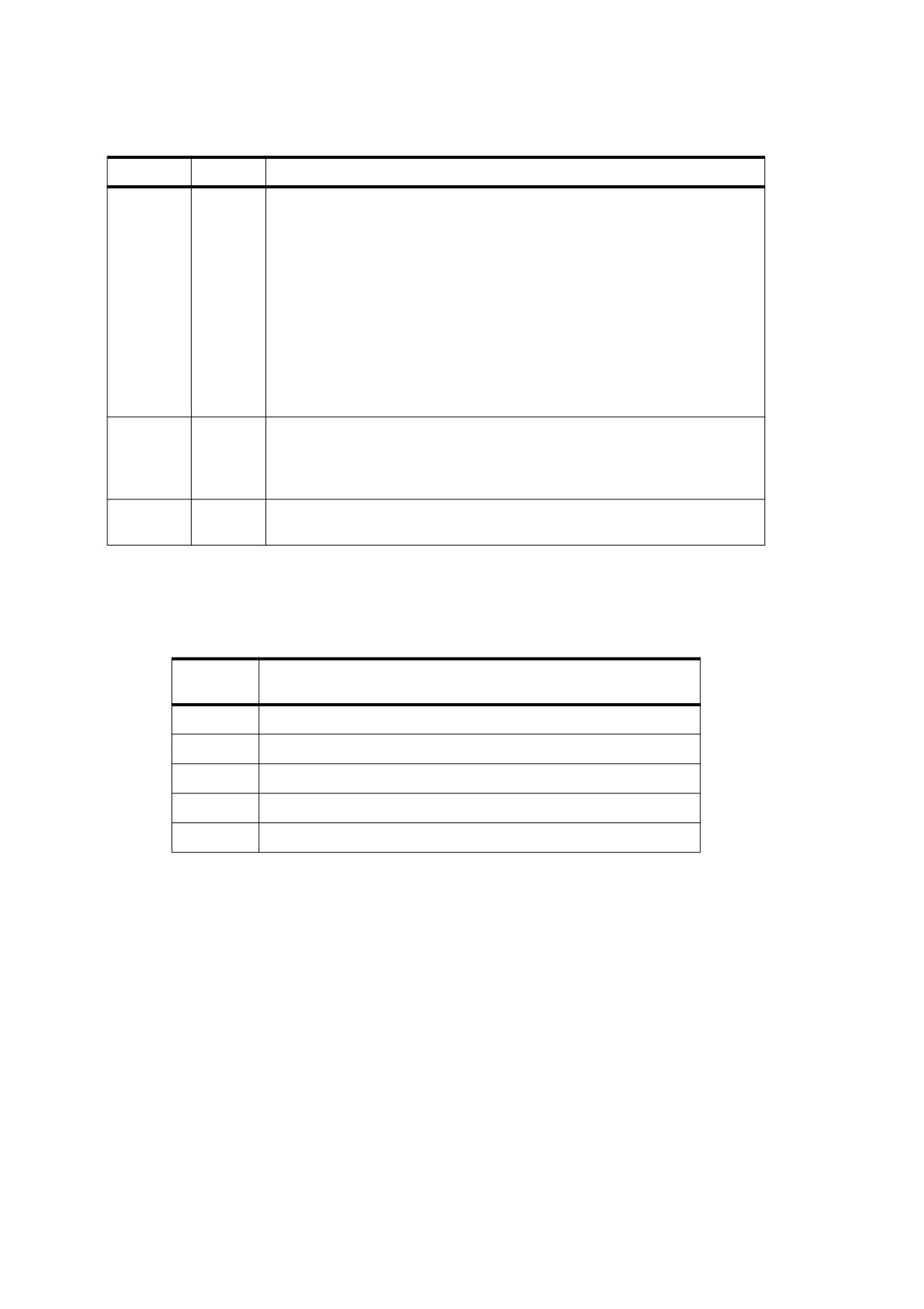
Table 66 - Additional Entries Specific to an ICC Profile Stream Dictionary (continued)

Key

Type

Value

Alternate

array or

(Optional) An alternate colour space that shall be used in case the one

name

specified in the stream data is not supported. Non-conforming readers may

use this colour space. The alternate space may be any valid colour space

(except a Pattern colour space) that has the number of components specified

by N. If this entry is omitted and the conforming reader does not understand

the ICC profile data, the colour space that shall be used is DeviceGray,

DeviceRGB, or DeviceCMYK, depending on whether the value of N is 1, 3, or

4, respectively.

There shall not be conversion of source colour values, such as a tint

transformation, when using the alternate colour space. Colour values within

the range of the ICCBased colour space might not be within the range of the

alternate colour space. In this case, the nearest values within the range of the

alternate space shall be substituted.

Range

array

(Optional) An array of 2 × N numbers [min₀ max₀ min₁ max₁ … ] that shall

specify the minimum and maximum valid values of the corresponding colour

components. These values shall match the information in the ICC profile.

Default value: [ 0.0 1.0 0.0 1.0 … ].

Metadata

stream

(Optional; PDF 1.4) A metadata stream that shall contain metadata for the

colour space (see 14.3.2, "Metadata Streams").

The ICC specification is an evolving standard. Table 67 shows the versions of the ICC specification on which

the ICCBased colour spaces that PDF versions 1.3 and later shall use. (Earlier versions of the ICC

specification shall also be supported.)

Table 67 - ICC Specification Versions Supported by ICC Based Colour Spaces

PDF

ICC Specification Version

Version

1.3

3.3

1.4

ICC.1:1998-09 and its addendum ICC.1A:1999-04

1.5

ICC.1:2001-12

1.6

ICC.1:2003-09

1.7

ICC.1:2004-10 (ISO 15076-1:2005)

Conforming writers and readers should follow these guidelines:

•

A conforming reader shall support ICC.1:2004:10 as required by PDF 1.7, which will enable it to properly

render all embedded ICC profiles regardless of the PDF version.

•

A conforming reader shall always process an embedded ICC profile according to the corresponding

version of the PDF being processed as shown in Table 67 above; it shall not substitute the Alternate colour

space in these cases.

•

A conforming writer should use ICC 1:2004-10 profiles. It may embed profiles conforming to a later ICC

version. The conforming reader should process such profiles according to Table 67; if that is not possible,

it shall substitute the Alternate colour space.

•

Conforming writers shall only use the profile types shown in Table 68 for specifying calibrated colour

spaces for colouring graphic objects. Each of the indicated fields shall have one of the values listed for that

field in the second column of the table. Profiles shall satisfy both the criteria shown in the table. The

terminology is taken from the ICC specifications.

150

NOTE 1

XYZ and 16-bit L*a*b* profiles are not listed.

Table 68 - ICC Profile Types

Header Field

Required Value

deviceClass

icSigInputClass ('scnr')

icSigDisplayClass ('mntr')

icSigOutputClass ('prtr')

icSigColorSpaceClass ('spac')

colorSpace

icSigGrayData ('GRAY')

icSigRgbData ('RGB ')

icSigCmykData ('CMYK')

icSigLabData ('Lab ')

The terminology used in PDF colour spaces and ICC colour profiles is similar, but sometimes the same terms

are used with different meanings. The default value for each component in an ICCBased colour space is 0. The

range of each colour component is a function of the colour space specified by the profile and is indicated in the

ICC specification. The ranges for several ICC colour spaces are shown in Table 69.

Table 69 - Ranges for Typical ICC Colour Spaces

ICC Colour Space

Component Ranges

Gray

[0.0

1.0 ]

RGB

[0.0

1.0 ]

CMYK

[0.0

1.0 ]

L*a*b*

L*: [ 0

100 ]; a* and b*: [ −128 127 ]

Since the ICCBased colour space is being used as a source colour space, only the “to CIE” profile information

(AToB in ICC terminology) shall be used; the “from CIE” (BToA) information shall be ignored when present. An

ICC profile may also specify a rendering intent, but a conforming reader shall ignore this information; the

rendering intent shall be specified in PDF by a separate parameter (see 8.6.5.8, "Rendering Intents").

The requirements stated above apply to an ICCBased colour space that is used to specify the source colours

of graphics objects. When such a space is used as the blending colour space for a transparency group in the

transparent imaging model (see 11.3.4, "Blending Colour Space"; 11.4, "Transparency Groups"; and 11.6.6,

"Transparency Group XObjects"), it shall have both “to CIE” (AToB) and “from CIE” (BToA) information. This is

because the group colour space shall be used as both the destination for objects being painted within the group

and the source for the group’s results. ICC profiles shall also be used in specifying output intents for matching

the colour characteristics of a PDF document with those of a target output device or production environment.

When used in this context, they shall be subject to still other constraints on the “to CIE” and “from CIE”

information; see 14.11.5, "Output Intents", for details.

The representations of ICCBased colour spaces are less compact than CalGray, CalRGB, and Lab, but can

represent a wider range of colour spaces.

NOTE 2

One particular colour space is the “standard RGB” or sRGB, defined in the International Electrotechnical

Commission (IEC) document Color Measurement and Management in Multimedia Systems and Equipment

(see, “Bibliography“). In PDF, the sRGB colour space can only be expressed as an ICCBased space,

although it can be approximated by a CalRGB space.

EXAMPLE

The following shows an ICCBased colour space for a typical three-component RGB space. The profile’s

data has been encoded in hexadecimal representation for readability; in actual practice, a lossless

decompression filter such as FlateDecode should be used.

10 0 obj

% Colour space

[ /ICCBased 15 0 R ]

151

Content      ..     2      3      4      5     ..