Content .. 1 2 3 4 ..

Technology of watch production - part 3

The difference between the maximum and minimum diameters , called

the r a n g e , will be equal to

act

-dmtn= 10.014-9.988

0.026

It.

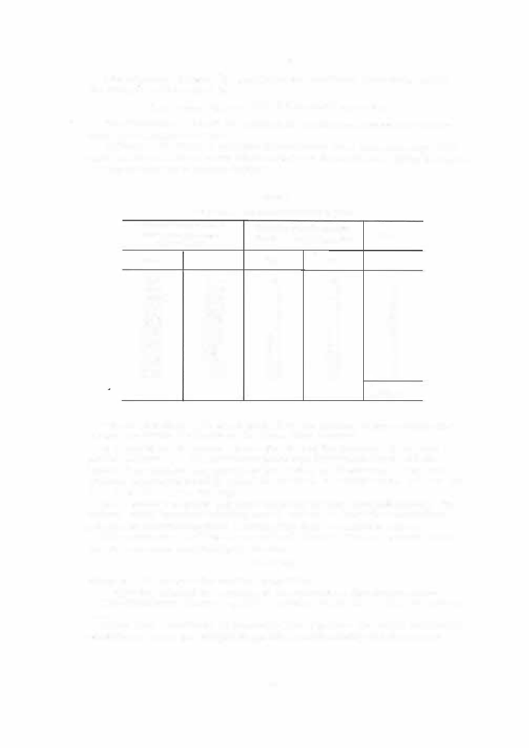
The diameter of each of the parts in the batch is measured and the re

sults are arranged in a table .

T o that end the range i s split into several equal class intervals , say, o f

211

each and the number of parts whos e measured diameter lies within the limits

of each interval is recorded ( Table 1

)

TABLE

Results of the measurement of a batch of parts

Class intervals of actual

diameter

(d1)in

increas-

ing order, mm

from

9 .988

9 .990

9.990

9 .992

9.994

9 ,996

9 .996

9 .998

10.000

10 .000

10 .002

10 .004

10.006

10 .006

10 .008

10.008

10.010

10 .010

10.012

10 .012

10 .014

Deviation from the nominal

diameter

�,=

d1-·anom' in�

from

-12

-10

- 8

-8

- 6

-4

- 4

- 2

-2

+10

+12

+14

Frequency

�

m1=

100

The f r e q u e n c y of a given interval is the number of parts whose dia

m eter lies within the limits of the given class interval .

A graph of the frequency

as a function of the deviation

131

can now be

plotted (Figure 1

)

. The points are connected by straight lines; and the

b roken line obtained characterizes the s catter of dim ensions in the batch

of parts investigated and is called the a c t u a l d i s t r i b u t i o n c u r v e o r
t h e d i s t r i b u t i o n p o

y g o n .

I f the number o f parts and class intervals i s increas ed indefinitely, the

interval width becomes infinitely small, and in the limit the dis tribution

polygon is transformed from a b roken line into a continuous curve .

This curve is called the t h e o r e t i c a

d i s t r i b u t i o n c u r v e and it

can be exp ressed analytically in the form

=<p(X),

where x

the value of the random magnitude;

<p(x)

the value of the ordinate of the continuous distribution curve .

The distribution function

'f'(x)

of a variate

is called the d i s t r i b u t i o n

l a w .

I t has been established by numerous investigations that under production

conditions , where the equipm ent operates automatically and there is no

dominating factor among the s ources of error, the s catter of errors in a

batch of parts conforms to or closely app roaches the law of normal distri

bution. This law is expressed analytically by the equation

-(X 1-xav)t

2•'

y =

y'21i

/il

- 'To'

=--e

Jf2Ti

where y

frequency of appearance of an error of given absolute value;

Xav

arithmetic mean of the actual dimensions (population mean ):

x1 =

actual dimensions;

the variable error;

a =

s tandard deviation, determined from one of the following expres

s ions :

fl,

12
10

8
G
4

FIGURE

1 .

Distribution polygon

1 0

The curve repres enting the law of normal distribution is given in Figure 2 .

The axis o f symmetry o f the curve is determined by

Xav•

which i s called

thepo p u l a t i o n m e a n .

The standard deviation

is the s econd main parameter of the law o f

no rmal distribution.

FIGURE

Curve of normal distribution

The larger the standard deviation, the broader and less s teep the curve .

A small value of a.on the contrary, will caus e the curve to be narrow and

steep.

We pres ent for comparison, in Figure 3 , three curves having different

values of

a .

A small value of

indicates small random errors , and a high

proces s ing accuracy. The value of

can therefore s erve as a criterium

of process accuracy.

FIGURE

Normal distribution curves with various values of "

1 1

The normal distribution curve has two inflection points , s ituated symme

trically on both sides of

at ±

The standard deviation ±a s eparates the region o f frequently met erro rs

from ·that of rarely met errors .

The branches of the normal distribution curve continue to infinity in both

directions and approach the X-axis asymptotically. The area under the curve

limited by the o rdinates ± 3 a includes 9 9 . 7 % of all the cases and therefore,

normal distribution curves are limited in practice to ±3o; this giving an

error of less than 0 . 3 % (Figure 2 ).

The accuracy with which the standard deviation can be determined de

pends on the number of parts measured.

For practical purposes it is wholly sufficient to determine the standard

deviation a with an error of ± 1 0 o/o, and in order to determine a to this de

gree of accuracy it is sufficient to m easure 50 parts .

Investigation of the A ccuracy of Technological Processes on the

Basis o f the Distribution Curve (Statistical Method)

Using the statistical m ethod, the manufacturing accuracy of a given pro

cess (the resultant error caus ed by the interaction of s e veral prim ary er
rors ) can be obtained, but the s eparate influence of each of these errors

cannot be directly obs erved .

The influenc e of a given factor can be determined by comparing distri

bution curves . If the distribution curve for the dim ens ions of a batch of

parts conforms to the law of normal distribution, the probability that the

error relative to the mean value in a part will not be larger than ± x0 (the

shaded area of Figure 4 ) will be

..-av+xo -(xi- Xav)2

---

I s

2a2

(J·

y2it

Xav-zo

d.x.

Instead of calculating the value of the integral corresponding to the spe

cified value of x0 in each instance , the table in A ppendix I can be us ed .

In this table the total area under the curve is taken as unity. The value

of z

is given in the firs t c olumn, and the values of the integral, de-

signa ted by

( z), are listed in the following columns . The values of z appear

in the first column to the first decimal place; the s econd decimal place ap

pears at the head of the following columns . Thus, for z

2 . 48;

( z) = 0 . 9868;

forx0

3a; <D(z) = 0. 9 9 7 3 or 9 9 . 7 3 % .

I f the probability is given, the value o f z can b e determined from the

formula z

and therefore the limiting deviation from the m ean value can

be calculated .

Thus , given a 1 . 5 % reject rate in a batch of parts , we obtain the value

z =

2.4 3

from the table for <D(z) = 0 . 9 8 5 .

Taking a

0 . 0 2 m m , w e will determine deviation

from the mean

value

Xav .

Content .. 1 2 3 4 ..