DB2 Server for VSE. Operations Guide / Handbooks (2004-2007)

If access is through an index, the proportion of pages read depends on the filter

factor for the predicates applied through the indexes and on the extent to which

the data rows are clustered by the index.

Using Explanation Tables to Evaluate Performance

The explanation tables produced by the EXPLAIN statement allow you to get

information about the structure and execution performance of SQL statements. This

information can help you analyze how existing database designs perform, or how

future designs will perform. Specifically, you can use explanation tables to:

v Find out the indexes that are used for a given statement, the number of index

columns used selectively, whether index-only access was sufficient to fulfill the

request, and whether a fetch operation was required

v Find out the sorts that are required, and the reason for the sorts

v Analyze request loads

v Estimate the size of responses

v Separate queries into their subquery structures

v Obtain costs for statements and access paths

v Assist in database design

v Determine when a program must be preprocessed again.

After you complete your design, and construct a prototype, you can use

explanation tables to see how well real queries will work against the design. (You

can select explain processing explicitly using the EXPLAIN statement, or implicitly

using the EXPLAIN(YES) preprocessing parameter or the USING EXPLAIN(YES)

option of the CREATE PACKAGE statement.)

Explain Processing

Explain processing accepts an SQL statement as an argument, analyzes it, and

inserts information about the structure and execution of that statement into the

explanation tables, that are created. (This includes the cost of internally generated

statements.) You can then query the explanation tables.

You can select explain processing explicitly by using the EXPLAIN statement, or

implicitly using the EXPLAIN(YES) preprocessor parameter or the EXPLAIN(YES)

USING OPTION of the CREATE PACKAGE statement or the EXPLAIN(YES)

option of the DBSU REBIND PACKAGE command.

Note: Explain processing does not execute the SQL statement. It only explains how

the statement will work when you actually execute it.

Using the EXPLAIN Statement

You can use the SQL EXPLAIN statement in an application program, the DBS

utility, or ISQL to estimate execution performance. For the syntax of the EXPLAIN

statement and the structure of the explanation tables produced, refer to the DB2

Server for VSE & VM SQL Reference manual.

To explicitly process the EXPLAIN statement, you must either:

v Preprocess the program every time you change the statement that EXPLAIN is

to analyze; or,

v Use multiple EXPLAIN statements; or,

v Have the program build the EXPLAIN statement and then execute it using the

dynamic prepare statements.

Chapter 5. Improving Data Access Performance

141

v Replace all the host variables with parameter markers and then issue an

EXPLAIN for it. For specific rules regarding the use of parameter markers, see

the DB2 Server for VSE & VM SQL Reference manual.

Each time the EXPLAIN statement is executed, rows are appended to the specified

explanation tables. Any existing rows are not affected.

When the EXPLAIN statement is issued for INSERT, UPDATE, and DELETE

statements that change tables in a referential structure, information is returned not

only on the INSERT, UPDATE, and DELETE statements, but also on internally

generated statements. Refer to the DB2 Server for VSE & VM Application

Programming manuals for more information on internally generated statements.

Each of the explanation tables has a column called QUERYNO (query number).

The QUERYNO column has a data type of INTEGER. With the SET QUERYNO

clause, you can place an integer value in the QUERYNO columns of the rows

inserted by the EXPLAIN statement. Thus, you can use QUERYNO to identify new

rows, and to mark them as corresponding to a particular statement.

For integer in SET QUERYNO, you must specify an integer constant that is not

preceded by a sign. You cannot use a host variable in the SET QUERYNO clause,

even in application programs. However, you can use the “&n” place-holder

variables in ISQL.

The SET QUERYNO clause is optional. If you omit it, a NULL value is placed in

the fields of the rows inserted by the EXPLAIN statement. If you set the

QUERYNO to some initial value, this value identifies the query for which the

EXPLAIN is issued. Because QUERYNO is an INTEGER field, an error is returned

if its value exceeds 2 147 483 647.

You can enter the EXPLAIN statement from ISQL. When you enter EXPLAIN from

ISQL, you must use a character constant if you execute the statement immediately.

Alternatively, you can store the EXPLAIN statement by placing it in a routine or

by using an ISQL STORE statement. This lets you use a place-holder (for example,

&1) for explainable_sql_statement (refer to the DB2 Server for VSE & VM SQL

Reference manual for the syntax of the EXPLAIN statement, including

explainable_sql_statement). Thus, you can execute EXPLAIN for different SQL

statements without having to key in the entire EXPLAIN statement each time.

When using this technique, however, you should keep ISQL limits in mind. For

example, when the place-holder is in a routine table, the length of input to a

parameter is limited by the length of the COMMAND column of the routine table.

At most, input to a place-holder can be 254 characters. This number is further

reduced if you do not put the “&n” place-holder on a line by itself.

When you enter EXPLAIN from the DBS utility, you must use a character

constant for explainable_sql_statement. The utility does not allow the use of host

variables or place-holders in any SQL statement.

Using the EXPLAIN Option

You can select explain processing implicitly using the EXPLAIN(YES)

preprocessing parameter or the EXPLAIN(YES) using option of the CREATE

PACKAGE statement or the EXPLAIN(YES) option of the DBSU REBIND

PACKAGE command. If you select explain processing implicitly, explanatory

information is provided for all internally generated SQL statements in a package.

The name of the package and the name of the owner of the package are stored in

the explanation tables.

142

Performance Tuning Handbook

You cannot assign a QUERYNO when you select explain processing implicitly and

hence the section number assigned to the statement being preprocessed is used as

the query number. This number corresponds to the position of the query in the

application. Using the preprocessor listing file, you can determine the section

number assigned to a statement and use it to determine the corresponding rows in

the explanation tables. The following variable names are used as section numbers

for the languages specified.

Table 9. Variable Names for Section Number (Query Number)

Language

Structure Name

Variable Name

ASM

RDIIN

RDISECT#

COBOL

RDIIN

SQL-SECTION-NUM

RDIIN

SECTION_NUM

PLI

RDIIN

SECTION_NUM

Fortran

SQLCTL

SQLSTMT

For further information, see the DB2 Server for VSE & VM SQL Reference and DB2

Server for VSE & VM Application Programming manuals.

Comparing Implicit and Explicit Explain Processing

Implicit and explicit explain processing insert the same kind of information into

the explanation tables during explain processing. The package name and package

owner columns of the explanation tables, however, contain information only if

implicit explain processing is used.

There is also a difference between implicit and explicit explain processing for the

query number of an application. For explicit explain processing, if you do not

supply the query number, it is set to NULL. For implicit explain processing, you

cannot provide query numbers for SQL statements in the middle of an application,

so the section number assigned to the statement when it is processed is used as the

query number. You can then use the preprocessor listing file to determine the

section number assigned to each statement and the corresponding rows in the

explanation tables.

During explicit explain processing, rows are added to the explanation tables when

a program is preprocessed, or dynamically repreprocessed. During implicit explain

processing, rows are added when a program is preprocessed, but not when it is

dynamically repreprocessed. In all situations, explicit explain processing overrides

implicit explain processing.

When you processes an application program using the implicit EXPLAIN(YES)

option, the preprocessor checks for the existence of the EXPLAIN tables once. If it

does not find them, processing is terminated and SQLCODE -649 (SQLSTATE =

42704) is issued.

Each time the preprocessor encounters an explicit EXPLAIN statement, it checks

for the existence of the explain tables. If its does not find them the explicit

EXPLAIN is not processed and, SQLCODE -204 (SQLSTATE = 42704) or

SQLWARNING +204 (SQLSTATE = 01532) is issued. This check is repeated for

every explicit EXPLAIN statement that the preprocessor encounters.

Using Explanation Tables

There are four explanation tables: REFERENCE_TABLE, STRUCTURE_TABLE,

COST_TABLE, and PLAN_TABLE. The definitions of these tables and the

Chapter 5. Improving Data Access Performance

143

EXPLAIN statement syntax are in the DB2 Server for VSE & VM SQL Reference

manual. A DBS utility job file, ARISEXP, to generate explanation tables, indexes,

and views is shipped with the DB2 Server for VSE & VM product. Instructions for

generating the tables using the ARISEXP file are provided at the top of the file. For

further information on the contents of the explanation tables, refer to the DB2

Server for VSE & VM SQL Reference manual.

When you execute an EXPLAIN statement, information is placed in your tables,

and is independent of any other user’s explanation tables. You can review and

summarize the information placed in your explanation tables just as you can other

tables. However, because explanation tables only insert rows, you also have the

responsibility to delete unnecessary information yourself.

In the following descriptions of each table, the term query block is used. A query

block is a part of a query. Query blocks are used to distinguish the parts of a

subquery. For example, when a query does not involve a subquery, there is only

one query block: query block 1. When there is a subquery, there are two query

blocks, the outer-level query and the subquery. They are referred to as query block

1 and query block 2, respectively. Because subqueries may be nested within each

other, there may be many query blocks in a statement; each query block

corresponds to separate (but interacting) parts of the statement.

The SELECT statement in Figure 17 is used in the following descriptions of the

explanation tables. This SELECT statement has only one query block.

SELECT X.DEPTNAME, Y.FIRSTNME, Y.MIDINIT, Y.LASTNAME, Y.PHONENO

FROM DEPARTMENT X, EMPLOYEE Y

WHERE X.MGRNO = Y.EMPNO

AND X.DEPTNO = Y.WORKDEPT

Figure 17. SELECT Statement for Explanation Table Descriptions

Assume that user Smith owns tables DEPARTMENT and EMPLOYEE where:

v DEPARTMENT has columns DEPTNO, DEPTNAME, MGRNO, and

ADMRDEPT.

v EMPLOYEE has columns EMPNO, FIRSTNME, MIDINIT, LASTNAME,

WORKDEPT, PHONENO, HIREDATE, JOB, EDLEVEL, SEX, BIRTHDATE,

SALARY, BONUS, and COMM.

Using the Cost Table: This table is updated by EXPLAIN COST or EXPLAIN

ALL. The information in this table provides the cost estimate of the statement for

which the EXPLAIN is issued and for any internally generated statement used to

enforce referential integrity. In addition, you can compute the contribution of each

subquery (if any) to the total cost estimate of the statement. (To compute the

subquery cost estimates, you will need to use information provided by the

EXPLAIN STRUCTURE statement.)

For each query block in the statement, EXPLAIN inserts one row into

COST_TABLE. The information depends on the existing indexes and catalog

statistics. If indexes are added or dropped after you issue EXPLAIN for the

statement, then the COST_TABLE entry for the command is not valid.

If you need a description of the columns in the COST_TABLE, refer to the DB2

Server for VSE & VM SQL Reference manual.

144

Performance Tuning Handbook

The value in COST is referred to as the cost estimate (occasionally referred to as

the optimizer cost estimate or the resource cost estimate). All of these terms refer

to the same thing: the internal value that the optimizer uses to represent the

resource cost of executing an SQL statement for which the EXPLAIN is issued and

for any internally generated statement used to enforce referential integrity. The

value is a relative value that incorporates I/O requirements with a weighted factor

of processor requirements for a query.

Aside from the COST column, there are two other ways to get this value for a

given SQL statement. One way is to examine the SQLCA after preparing a

dynamically defined SQL statement. The cost estimate is kept in the SQLERRD(4)

field. A second way to see the cost estimate is using ISQL. ISQL displays the query

cost estimate integer. The integer results from dividing the real internal value by

1000 and adding 1 to it. This produces a number that is easier to grasp. This is a

valid technique because the numbers are relative to each other; they do not

represent real physical consumption directly.

It follows, then, that it is futile to try to develop an algorithm that directly maps

the cost estimate to a real physical unit such as time. Too many other factors are

involved (for example, overall system workload). It is best to use the cost estimate

as a general indicator.

For the SELECT statement in Figure 17, there would be only one row entered into

COST_TABLE, because there is only one query block:

QUERYNO RINO QBLOCKNO PKGNAME PKGOWNER COST

-------

----

--------

-------

--------

------------------

1.4388885498046E+01

TIMESTAMP

--------------------------

1999-08-26-09.49.25.601721

Figure 18. Results of COST_TABLE Query

Using the Plan Table: This table is updated by EXPLAIN PLAN or EXPLAIN

ALL. The information in this table describes the order in which tables are accessed

by the statement for which the EXPLAIN is issued and by any internally generated

statement used to enforce referential integrity. In addition, the PLAN_TABLE table

describes the indexes used to access the tables, and specifies whether indexes alone

were used, the methods that the database manager used to do joins, the sorts done

as part of runtime processing, and the reasons for the sorts.

As with the COST_TABLE, the PLAN_TABLE results depend on the existing

indexes and catalog statistics at the time the EXPLAIN statement is executed. If

indexes are added or deleted, then the PLAN_TABLE entry for the statement is not

valid.

For each step in the plan determined by the database manager for processing the

query, EXPLAIN inserts one row into the PLAN_TABLE. There is one step for each

table reference in a query block. There are additional steps if the database manager

must perform additional sorts at the end of processing for the query block, or if

any internally generated statements are to be processed.

The steps in the plan are ordered by the value of the PLANNO column of

PLAN_TABLE, and for each step, the TNAME column identifies the table accessed.

The phrase “previous steps of the plan” refers to PLAN_TABLE rows with smaller

Chapter 5. Improving Data Access Performance

145

values of PLANNO. The action described in a step is either a join of a table to

those previously joined, or it is a sort. (Joins themselves may involve performing

sorts.) The term “composite” refers to the result of all previous steps; the term

“new” refers to the new table that is being accessed and joined as part of a

particular plan step.

If you need a description of the columns in the PLAN_TABLE, refer to the DB2

Server for VSE & VM SQL Reference manual.

The PLAN_TABLE for the query in Figure 17 is shown below. Because there are

many columns in PLAN_TABLE, the display of the table is split to fit on the page:

QUERYNO RINO QBLOCKNO PKGNAME PKGOWNER PLANNO METHOD CREATOR

-------

----

--------

-------

--------

------

-------

SMITH

TNAME

TABNO ACCESSTYPE MATCHCOLS ACCESSCREATOR

----------

-----

----------

---------

-------------

DEPARTMENT

SMITH

EMPLOYEE

SMITH

ACCESSNAME

INDEXONLY SORTNEW SORTCOMP SORTN_UNIQ SORTN_JOIN

----------

---------

-------

--------

----------

MGRNOI

PKEYB1H9ZR8CD51W

SORTN_ORDERBY SORTN_GROUPBY SORTC_UNIQ SORTC_JOIN SORTC_ORDERBY

-------------

----------

-------------

SORTC_GROUPBY TIMESTAMP

REMARKS

-------------

--------------------------

-------

1999-08-26-09.49.25.601721

Figure 19. Results of PLAN_TABLE Query

A Type 1 (or nested loop) join is performed on tables EMPLOYEE and

DEPARTMENT. The database manager accesses DEPARTMENT as the outer table

of the join (the first table accessed), and EMPLOYEE as the inner table of the join.

The row with PLANNO=1 indicates that the database manager accesses

DEPARTMENT using the index MGRNOI (which, as it happens, was created on

the MGRNO column).

The entry with PLANNO=2 indicates that the database manager has performed an

action on the EMPLOYEE table, based upon the conditions included in the query.

An index has been generated internally on the primary key EMPNO of the

EMPLOYEE table. This index performs the matching of EMPNO (in the

EMPLOYEE table) to MGRNO (in the DEPARTMENT table). This index can be

used because the value in MGRNO of DEPARTMENT, which must be matched by

the EMPNO value of EMPLOYEE. Retrieval of rows from an inner table of a join

will often, though not always, use an index on a join column of the inner table.

146

Performance Tuning Handbook

No sorts are used in the plan for this query. However, if the query had demanded

SELECT DISTINCT, instead of SELECT, the plan would have an additional row,

with PLANNO=3, which would have TABNO=0, METHOD=3, SORTC_UNIQ=‘Y’

and SORTCOMP=‘U’.

Using the Reference Table: This table is updated by EXPLAIN REFERENCE or

EXPLAIN ALL. The database manager inserts one row in REFERENCE_TABLE for

each column referenced in the statement (in certain ways, as explained below) and

for any internally generated statement used to enforce referential integrity. Even if

the column is referenced more than once for a table, there is still only one row

inserted for the column and that row is for the most selective predicate. However,

multiple appearances of a table in a query (as when a table is joined to itself) can

lead to multiple descriptions of their columns.

One row is entered for each table reference, one for the statement as a whole, and

one that indicates the way in which the column is used in the query. For a

description of the columns in the REFERENCE_TABLE, refer to the DB2 Server for

VSE & VM SQL Reference manual.

For the example statement presented in Figure 17 on page 144, the new rows

entered into REFERENCE_TABLE by EXPLAIN REFERENCE might be:

Chapter 5. Improving Data Access Performance

147

QUERYNO RINO QBLOCKNO PKGNAME PKGOWNER REFTYPE CREATOR

TNAME

-------

----

--------

-------

--------

-------

----------

SELECT

TABLE

SMITH

DEPARTMENT

TABLE

SMITH

EMPLOYEE

COLUMN

SMITH

DEPARTMENT

COLUMN

SMITH

DEPARTMENT

COLUMN

SMITH

DEPARTMENT

COLUMN

SMITH

EMPLOYEE

COLUMN

SMITH

EMPLOYEE

COLUMN

SMITH

EMPLOYEE

COLUMN

SMITH

EMPLOYEE

COLUMN

SMITH

EMPLOYEE

COLUMN

SMITH

EMPLOYEE

TABNO CNAME COLNO

FILTER

DBSSPRED

JOINPRED

ORDERCOL

-----

-------------------

--------

0.0E0

DEPTNAME

1.0E+00

DEPTNO

1.111111448837E-01

MGRNO

3.125E-02

EMPNO

3.125E-02

FIRSTNME

1.0E+00

LASTNAME

1.0E+00

MIDINIT

1.0E+00

PHONENO

1.0E+00

WORKDEPT

1.1111110448837E-01

GROUPCOL UPDATECOL

TIMESTAMP

--------

---------

-------------------------

1999-08-26-09.49.25.601721

Figure 20. Results of the REFERENCE_TABLE Query

These rows indicate that the statement is a SELECT statement with no subqueries,

joining two tables, SMITH.DEPARTMENT and SMITH.EMPLOYEE. The columns

MGRNO, DEPTNO from DEPARTMENT, and the columns EMPNO, WORKDEPT

from EMPLOYEE appear together in the 'WHERE' clause (identified by a Y in the

DBSSPRED column), permitting indexes to be used. These columns are the JOIN

columns (identified by a Y in the JOINPRED column). FILTER may be misleading,

because the filtering depends on the order in which tables are processed.

148

Performance Tuning Handbook

Referential Integrity (RINO Value)

RINO is set to zero for the original statement and is automatically incremented by one for each

internally-generated statement that is processed for referential integrity or cascade delete. For example if you

perform an EXPLAIN against a statement that deletes a department from the DEPARTMENT table, the

following REFERENCE table is generated.

QNO RINO QBLOCK REFTYPE TNAME

CNAME

----------- ------ ------ ------- ------------------ ------------------...

0 DELETE

1 TABLE DEPARTMENT

0 UPDATE

1 TABLE EMPLOYEE

1 COLUMN EMPLOYEE

WORKDEPT

0 SELECT

1 TABLE PROJECT

1 COLUMN PROJECT

DEPTNO

Notice that the DELETE statement that was written (RINO=0) produces two other statements: First an UPDATE

that changes the WORKDEPT column for any employee in the deleted department to NULL (RINO=1), and

second a SELECT that checks that any departments to be deleted do not have any projects assigned to them

(RINO=2).

The REFERENCE_TABLE and the PLAN-TABLE can be used together to indicate whether materialization was

used to generate a view. View materialization lifts a number of restrictions on the use of views, including the

use of column functions operating on the column of a view when the definition of the view already contains a

column function. For example:

CREATE VIEW V1(DPT,MAXSAL) AS

SELECT WORKDEPT, MAX(SALARY)

FROM

EMPLOYEE

GROUP BY WORKDEPT

EXPLAIN ALL FOR SELECT DPT FROM V1

Because view materialization is used for view V1, the TNAME column in the REFERENCE_TABLE and

PLAN_TABLE will contain the name of the view. Keeping in mind that view materialization is generally more

expensive than merging the SELECT statement of the view with that of the query, the information on the

EXPLAIN tables can be helpful in performance tuning.

Using the Structure Table: This table is updated by EXPLAIN STRUCTURE or

EXPLAIN ALL. The database manager inserts one row in STRUCTURE_TABLE for

each query block in the statement.

If you need a description of the columns in the STRUCTURE_TABLE, refer to the

DB2 Server for VSE & VM SQL Reference manual.

If the following SELECT statement is issued, only one row is entered in

STRUCTURE_TABLE, as shown in Figure 21 on page 150, because there is only one

query block.

EXPLAIN ALL FOR SELECT * FROM EMPLOYEE

Chapter 5. Improving Data Access Performance

149

QUERYNO RINO QBLOCKNO PKGNAME PKGOWNER ROWCOUNT

TIMES

-------

----

--------

-------

--------

---------

0.0E0

PARENT ATOPEN TIMESTAMP

------

--------------------------

1999-08-26-09.49.26.001720

Figure 21. Results of the STRUCTURE_TABLE Query

A more complicated example is provided in the following sections, where we show

how to separate the costs for individual query blocks using STRUCTURE_TABLE

and COST_TABLE together.

Using Subquery Blocks: A query may have subqueries, which in turn may have

subqueries. The database manager separates this tree of subqueries into pieces,

called query blocks. Each query block has its own tables, columns, and rowcount.

EXPLAIN STRUCTURE, COST lets you look at combined information, or to

separately examine the information for each query block.

The PARENT field gives the logical parent for each query block, which is not

always obvious from the query itself. Sometimes, a query block has no correlation

to the query where it immediately appears, so it is executed only once, when some

ancestor query block is first entered, rather than many times.

The following example has a large number of query blocks, but references only one

table (many times). It illustrates the meanings of PARENT and ATOPEN, as well as

the method for decomposing COST values into separate costs for query blocks.

QBLOCKNO

---------

SELECT * FROM DEPT X

*** 1 ***

WHERE DNAME > ALL

(SELECT DNAME FROM DEPT

*** 2 ***

WHERE X.DNO = DNO

AND LOC = 32)

AND DNO =

(SELECT DNO FROM DEPT Y

*** 3 ***

WHERE MGR =

(SELECT MGR FROM DEPT Z

*** 4 ***

WHERE DNAME IN

(SELECT DNAME FROM DEPT

*** 5 ***

WHERE NEMP = X.NEMP)

AND DNO =

(SELECT DNO FROM DEPT W

*** 6 ***

WHERE NEMP > Z.NEMP

AND LOC IN

(SELECT LOC FROM DEPT

*** 7 ***

WHERE DNAME = Y.DNAME))

AND LOC = 32 )

AND Y.NEMP <

(SELECT AVG(NEMP) FROM DEPT

*** 8 ***

WHERE Y.MGR = MGR ));

Here are results from STRUCTURE_TABLE for this query. (ROWCOUNT is not

shown.)

150

Performance Tuning Handbook

QUERYNO RINO QBLOCKNO PKGNAME PKGOWNER TIMES PARENT

-------

----

--------

-------

--------

------

9.000

0.500

9.000

0.500

2.000

1.500

1.000

ATOPEN TIMESTAMP

------

--------------------------

1999-08-26-09.49.27.011719

Figure 22. Example STRUCTURE_TABLE

Note: A ? indicates a NULL value.

Although query block 5 is physically nested within query block 4, it references

neither Y nor Z. Hence, its value can be computed once each time query block 3

first entered, with a particular X row.

Query block 5 is executed once, at open time of query block 3.

Query block 7 is physically within query block 6, but can be evaluated once when

the database manager first enters query block 4. Query block 7 does not need to be

re-executed again until new values for rows outside query block 4 are required.

This is different from query block 2, for example, which must be executed once for

each row of query block 1, rather than just once when execution of query block 1

begins.

TIMES may be a fraction (and may be less than 1) because it represents the

estimated number of times, per execution of a query block, that its dependent

query blocks will be executed.

The most important use of this query block breakdown involves computation of

costs for individual query blocks, instead of costs for the query as a whole. This is

described next.

Computing Block Costs: Here are the COST_TABLE entries for the query in the

preceding section:

Chapter 5. Improving Data Access Performance

151

QUERYNO RINO QBLOCKNO PKGNAME PKGOWNER

COST

-------

----

--------

-------

--------

---------

3021.000

10.000

324.000

24.000

4.000

6.000

10.000

TIMESTAMP

--------------------------

1999-08-26-09.49.27.011719

Figure 23. Results of COST_TABLE Query

The cost displayed is the total cost for each query block, including costs associated

with all query blocks that are below it in the logical tree of query blocks. Thus, the

cost of executing the statement is approximately 3021. (For simplicity in the

calculations that follow, the values are shown as integers, but they need not be.)

The cost for executing the entire statement helps you understand the effect of the

statement on system load, but it hides the blocks of the query that are contributing

the most to the cost of the query.

A more useful set of figures might be those listed in the following table:

Note: The following table is only an example. It is not stored in the database, and

INDIVCOST and MULTCOST are not columns in COST_TABLE.

QBLOCKNO INDIVCOST

MULTCOST

--------

---------

----------

15.000

10.000

90.000

14.000

126.000

11.000

891.000

4.000

36.000

6.000

243.000

10.000

810.000

10.000

810.000

Figure 24. Example COST_TABLE

INDIVCOST represents the cost of one execution of the individual query block

itself, not including the costs of any of its subqueries. MULTCOST not only counts

the cost of the individual query block, but multiplies INDIVCOST by the number

of times the query block is expected to be executed in the query. This is a better

measure of the cost importance of the query block than either COST or

INDIVCOST. Notice that the MULTCOST column adds up to COST(1), the total

cost of the entire query.

152

Performance Tuning Handbook

Thus, the following formula can be used to derive INDIVCOST:

COST(I) = INDIVCOST(I) + the sum, over all blocks J that have

I as logical parent, of either:

TIMES(I) * COST(J)

if J is not done AT OPEN of I, or

COST(J)

if J is done AT OPEN of I.

For example:

COST(3) = 324 = INDIVCOST(3) + 9*24 + 4 + 9*10,

so INDIVCOST(3) is 14.

Here is another example:

COST(4) = 24 = INDIVCOST(4) + 0.5*6 + 10,

so INDIVCOST(4) is 11.

This formula can be used to derive MULTCOST from INDIVCOST:

MULTCOST(I) =

INDIVCOST(I) * the product of TIMES(I) for

all logical ancestors of I,

if I is not done AT OPEN of its parent,

INDIVCOST(I) * the product of TIMES(I) for

all logical ancestors of I EXCEPT its parent,

if I is done AT OPEN of its parent.

For example:

MULTCOST(7) = 10 * TIMES(3) * TIMES(1) = 810.

We do not multiply TIMES(4) into that product, because 4 is 7’s immediate parent,

and 7 is done AT OPEN of 4.

This demonstrates that the most important component of the estimated cost comes

from block 4, and you might choose indexes that make processing this query block

cheaper. By inspecting the query, or from the rows in REFERENCE_TABLE, you

might decide that indexes on one of DNAME, DNO or LOC might reduce the cost

of processing.

Estimating Sizes of Responses

Because ROWCOUNT (estimated number of rows in result, for queries, or of

affected rows, for updates and deletes) is stored in STRUCTURE_TABLE, it is easy

to gauge the estimated size of responses. If your structure includes a DELETE

Chapter 5. Improving Data Access Performance

153

CASCADE rule, EXPLAIN will include the cost of the cascading effects of a

DELETE. This can help you understand whether requests are reasonable, and

whether the statistics in the database catalog tables that estimate ROWCOUNT

seem up-to-date.

ROWCOUNT can also help determine space requirements when responses are

being stored in program data structures. However, ROWCOUNT, like all estimates

made by the system, is neither precisely accurate, nor even an upper bound on the

actual number of rows in the response.

Using EXPLAIN for Database Design

A systematic analysis of many statements in the workload of the system can help

the administrator plan the access paths for the database. The analysis should

consider costs when different combinations of indexes exist. It should also consider

the costs of performing updates, which are not reflected in the COST column of

COST_TABLE, and limits on space for indexes.

You may load the database with tables ordered on certain columns. Indexes on

such columns (called CLUSTERING indexes) enable the database manager to

maintain this ordering. Because the ordering of rows within tables strongly affects

the costs of execution, it may be worthwhile to reload the database to improve

performance. For each statement, join, ORDER BY, and GROUP BY columns may

be good candidates for ordering. Also, tables that are often joined might be

interleaved on join columns when the database is loaded.

If the cost of executing a statement (as determined by EXPLAIN COST, or by

running the statement) is higher than expected, a user or administrator may want

to look at the procedure that the database manager chose to execute that statement.

Building additional access paths or altering the layout of tables may be necessary

to achieve good performance for the statement. For example, if a relation scan, that

is ACCESS TYPE=‘R’, is performed on a large table, it may be better to build an

index on some column of that table; EXPLAIN REFERENCE provides hints about

which indexes might help. Adding new indexes makes updates more expensive, so

this decision must be considered carefully.

The PLAN_TABLE can also help the administrator determine which indexes are

not being used, so that he or she may decide which indexes might be dropped.

This assumes that the administrator knows not only the significant statements in

programs, but also the significant statements issued by users directly at their

terminals.

Modifying Table Designs to Enhance Performance

The primary consideration for the performance of access to data in the database is

the number of DASD input/output requests required to access the table rows. The

indexing and clustering techniques discussed in the previous sections enhance data

access performance by reducing DASD input/output requests without impacting

your logical data (table) design. However, other techniques can be used, if you are

willing to reconsider your logical table design.

Keeping Together Frequently Updated Columns: Keep frequently updated columns

close together in the same row. This helps to reduce the amount of data that has to

be logged because only the portion of the row from the first column updated to

the last column updated is recorded in the log.

154

Performance Tuning Handbook

Storing Joins of Tables (Redundant Data): The evaluation of a join of two tables

involves combining information from corresponding rows of the tables. Ideally, the

corresponding rows are on the same page. However, such clustering of rows from

separate tables is difficult to establish and maintain. Then, such clustering may not

be in the best interest of query accesses to the individual tables. Assuming tables

are clustered on different pages, multiple input/output requests are required to

evaluate the join of corresponding rows of the two tables.

For example, suppose the PROJECT table is clustered on DEPTNO. Retrieving

information about a department (a DEPARTMENT row) and its corresponding

project name (PROJECT rows), involves an access to one page to get the

DEPARTMENT row and another access to a different page to get the

corresponding PROJECT rows.

If most of such joins are done just to pick up the DEPTNAME information out of

the DEPARTMENT row, it may be worthwhile to store DEPTNAME in both tables.

This eliminates the need to join the two tables to obtain department names

(DEPTNAMEs) in retrieval of project names. This, in turn, eliminates accesses to

the DEPARTMENT table pages. This, in effect, reduces database input/output

requests by “storing the join” of the two tables.

You can use the ISQL INSERT with Subselect (Format 2) to combine tables.

The extreme case of “storing joins” is to replace both tables with the complete join

(SELECT *) of the two tables. This is rarely cost effective.

The cost of storing joins is the DASD space consumed and the extra activity

required to maintain the redundant data. Table 10 shows the cost of storing the

DEPTNAME column in the PROJECT table.

Table 10. Cost of Storing DEPTNAME in the PROJECT Table

Cost Factor

Approximate Cost

DASD Storage

The average column length of the DEPTNAME values

times the number of rows in PROJECT (approximately

20-bytes per PROJECT row) or approximately a 35%

increase in the average row length for PROJECT

INSERT into PROJECT

This requires the application to first access the PROJECT

table to obtain the DEPTNAME for inclusion in the

PROJECT row.

UPDATE of DEPTNAME

This requires an update to the PROJECT table (but this is

not a frequent operation).

DELETE of a PROJECT

No extra cost.

DELETE of a DEPTNAME No extra cost.

The cost of storing the DEPTNAME information redundantly is not excessive when

compared to the input/output cost for frequent selecting of department names

with queries on project information. The cost of DASD storage looks high (about a

35% increase in the size of the PROJECT table). However, a dbspace page will still

hold about 140 PROJECT rows. Because most departments have less than 140

project names, it is still reasonable to expect all project names for a department to

be on the same page for most departments.

Storing a Logical Table as Two Tables: Another way to reduce the number of

pages occupied by a table is to reduce the size of the table. There is not much you

Chapter 5. Improving Data Access Performance

155

can do to make a table smaller than it really is; however, you can achieve a similar

effect by separating frequently used columns from the infrequently used columns.

You can do this by splitting the table into two (or more) tables. One table would

contain the frequently used columns and the other(s) would contain the

infrequently used columns. You could then cluster the rows of frequently used

columns on a fewer number of pages.

The cost of splitting a table is the overhead added to queries that need all columns

(which, by definition, is infrequent). Splitting a table also produces redundant data.

That is, both (all) tables would have to contain the necessary column(s) to support

the join.

156

Performance Tuning Handbook

Chapter 6. Data Spaces Support for VM/ESA

Read this chapter before you implement VM Data Spaces Support (VMDSS). It

briefly describes the concept of data spaces, how they work, and how they can

improve performance; it outlines what options you have as a VMDSS user; and it

lists the prerequisite hardware and software.

Improving DB2 Server for VM Performance

VMDSS can dramatically increase the performance of your application server, by

using the Data Spaces facility found in VM/ESA. Data spaces give your

application server access to vast amounts of fast storage, and uses a high

performance DASD I/O system that has many advantages over the standard I/O

system (IUCV *BLOCKIO).

VMDSS can also distribute data across multiple dbextents, which helps to balance

the load on your system’s DASD and allows the operating system to read and

write data in parallel. Finally, you can monitor the performance of your DASD I/O

system for individual storage pools, and control the amount of system-resource it

uses.

Understanding VM Data Spaces

To understand how data spaces work and why they are an improvement over

existing systems, you first need to understand how VM uses its paging system to

manage virtual machine storage.

Standard Virtual Machine Storage

Each virtual machine within a VM system has its own virtual address space (also

called a primary address space) which is where you load and run programs.

Because this space is virtual, the operating system does not dedicate a piece of

main storage (also called real storage) to each virtual machine. You do not need to

buy 16MB of main storage for each 16MB virtual machine. Instead the operating

system only uses main storage for those parts of virtual storage you need right

now, or are likely to need in the near future.

These parts of storage are divided into 4KB (4096 byte) blocks called pages. When a

virtual machine needs a page that it has not accessed before, the operating system

retrieves it from its location on DASD, and loads it into an empty page in main

storage. (Before a virtual machine can use a page, it must be in main storage.)

When the operating system runs out of free pages in main storage, it moves the

least recently used (“oldest”) page to auxiliary storage to create a free space for a

new page. While the virtual machine is still active (logged on), the page will

remain in either main or auxiliary storage.

VM/ESA uses two types of auxiliary storage: system paging DASD, and optional

expanded storage. If your system has expanded storage, a page will be moved

there first. If expanded storage is full, the least recently used page in expanded

storage is moved to system paging DASD by way of main storage. When a virtual

machine needs a page that it has previously used, the operating system moves it

back to main storage from expanded storage, or from system paging DASD, if it is

157

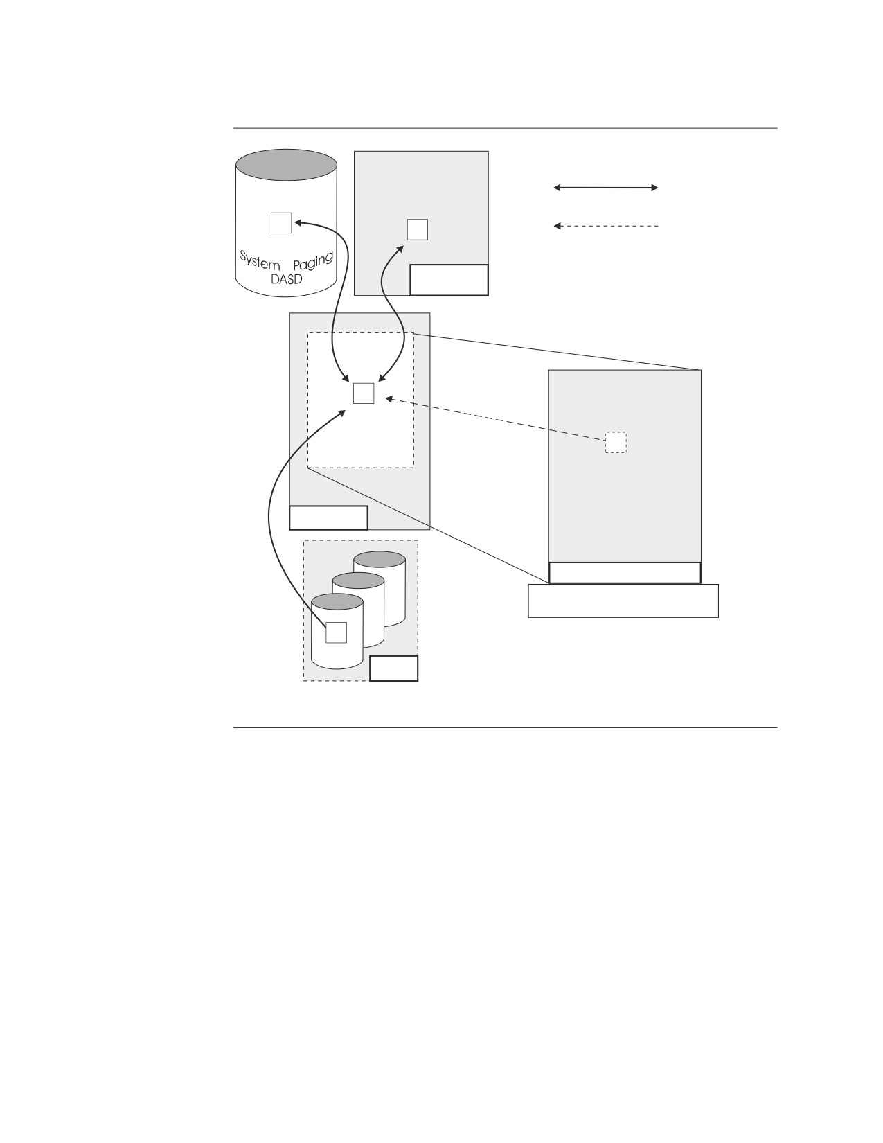
not already in main storage.

Physical Move

Pointer From Virtual

to Physical Page

Expanded

Storage

Main Storage

Virtual Machine

Control Program

(CP)

DASD

Physical Storage

Virtual Storage

Figure 25. Standard Virtual Machine Storage

This paging system accomplishes two things. First, it allows each virtual machine

to use much more storage than could be accommodated in main storage alone.

Second, it keeps the most recently used pages in the storage devices that are the

fastest to access. (The most recently used pages are the ones most likely to be used

again in the near future.) Main and expanded storage are much faster than system

paging DASD, and while expanded storage can be as fast as main storage, it is

effectively slower because the operating system still needs to move the page into

main storage before it can use it.

Data Spaces Storage

In VM/ESA, a program running in a machine’s primary space can dynamically

create additional address spaces for data, called data spaces. Like a virtual

machine’s primary address space, a data space is a virtual space with its real pages

in main storage, in expanded storage, and on DASD. However, unlike a primary

space, you cannot run a program in a data space. Also, in VMDSS the VM paging

system manages data space pages differently than virtual machine pages. This

means that data spaces do not use system paging DASD. (Unmapped internal

158

Performance Tuning Handbook

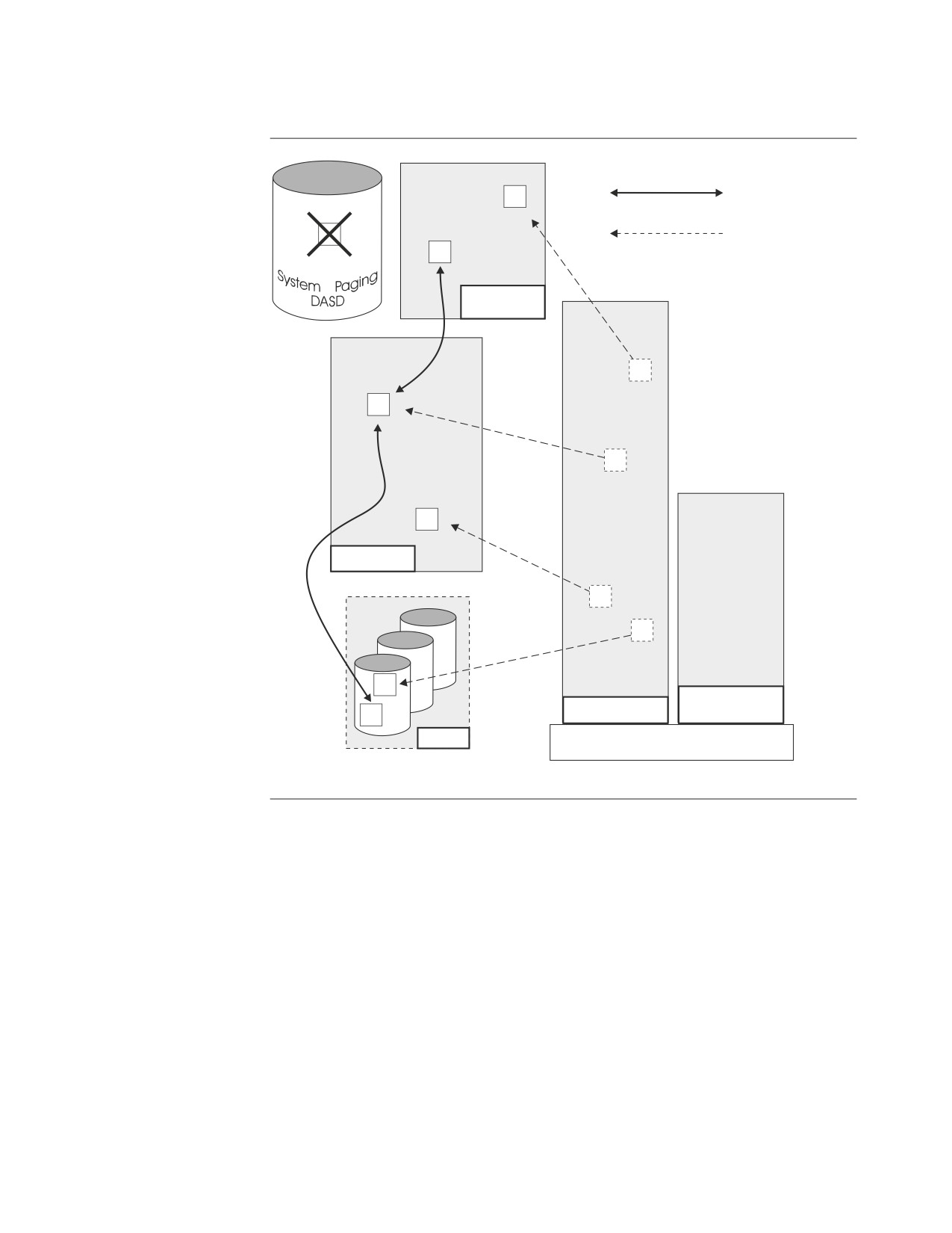
dbspaces are the exception. Refer to “Unmapped Internal Dbspaces” on page 164).

Physical Move

Pointer From Virtual

to Physical Page

Expanded

Storage

Main Storage

Virtual

Data Space

Machine

DASD

Control Program

(CP)

Physical Storage

Virtual Storage

Figure 26. Data Spaces Storage

With VMDSS, if there is no longer any free space in main or expanded storage, the

operating system will simply replace an old data space page in main or expanded

storage with a new page. If the old page is needed again, it is reread from its

original DASD source. If the old page was modified while it was in main storage,

the operating system ensures that the modified page is written back to its original

DASD source before it is overwritten.

This expands a machine’s effective virtual storage by providing additional

addresses for data, thereby making room in the primary space for larger programs.

Understanding how VMDSS uses Data Spaces

Reading Pages

Before a page of data can be used by the database manager, it must be located in

its data page buffers. The buffers are two areas of storage in your primary address

space, which are created when you start the database manager. One area is

Chapter 6. Data Spaces Support for VM/ESA

159

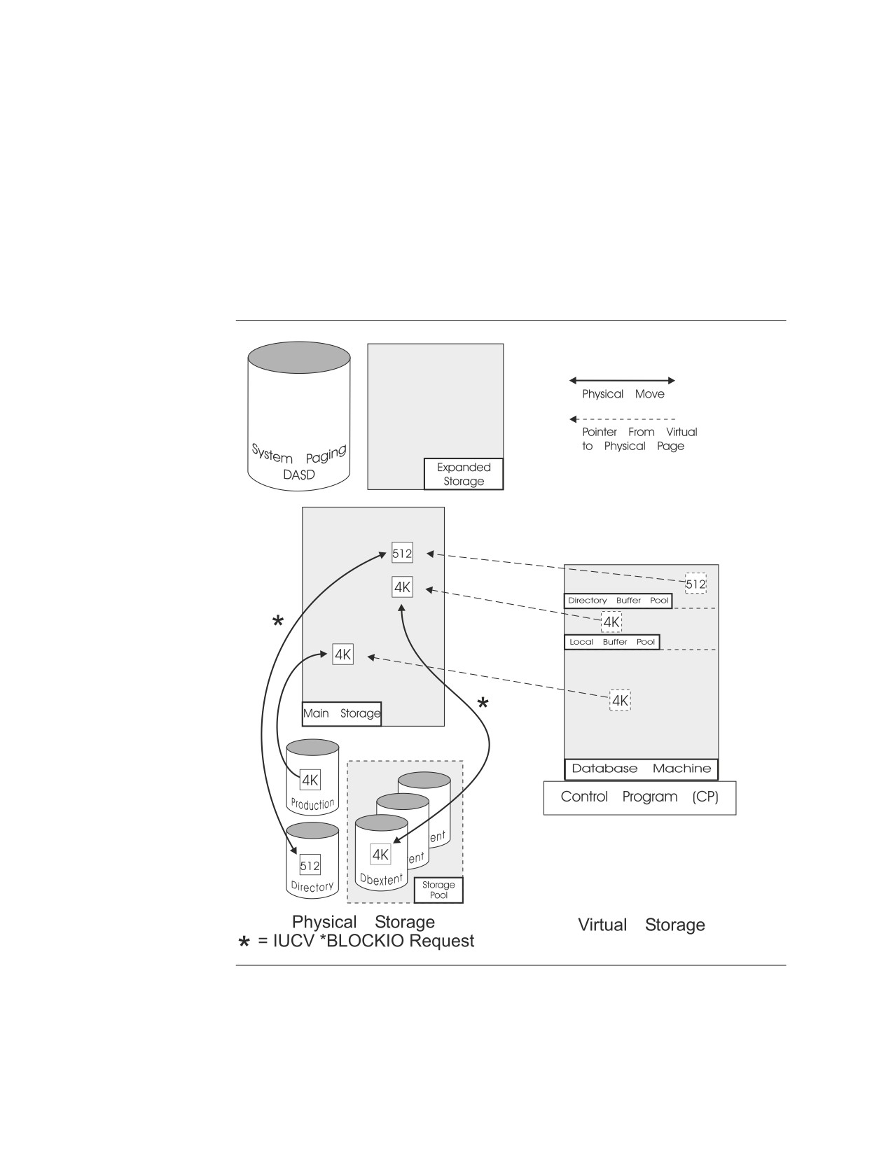
reserved for pages from the directory disk, and the other for pages from storage

pools. They are called the directory buffer pool and the local buffer pool, respectively.

With Data Spaces Support off: When the database manager needs a page, it

looks for it in its buffer pool. If it does not find it there, it uses a VM service called

IUCV *BLOCKIO to read the page from DASD into a free space in its pool.

Since the buffer pools are part of a primary address space, the operating system

treats them like part of the database manager code. If a buffer page is not

referenced frequently, it may be moved out to expanded storage or system paging

DASD by the VM paging system (for more information refer to “Asynchronous

Page Fault Processing” on page 197).

Figure 27. Page Movement in the Standard DASD I/O System. The database manager

explicitly directs the operating system to move pages to and from DASD with the IUCV

*BLOCKIO instruction. Once database machine pages are in main storage, they may be

moved out to either expanded storage or system paging DASD by the VM paging system.

160

Performance Tuning Handbook

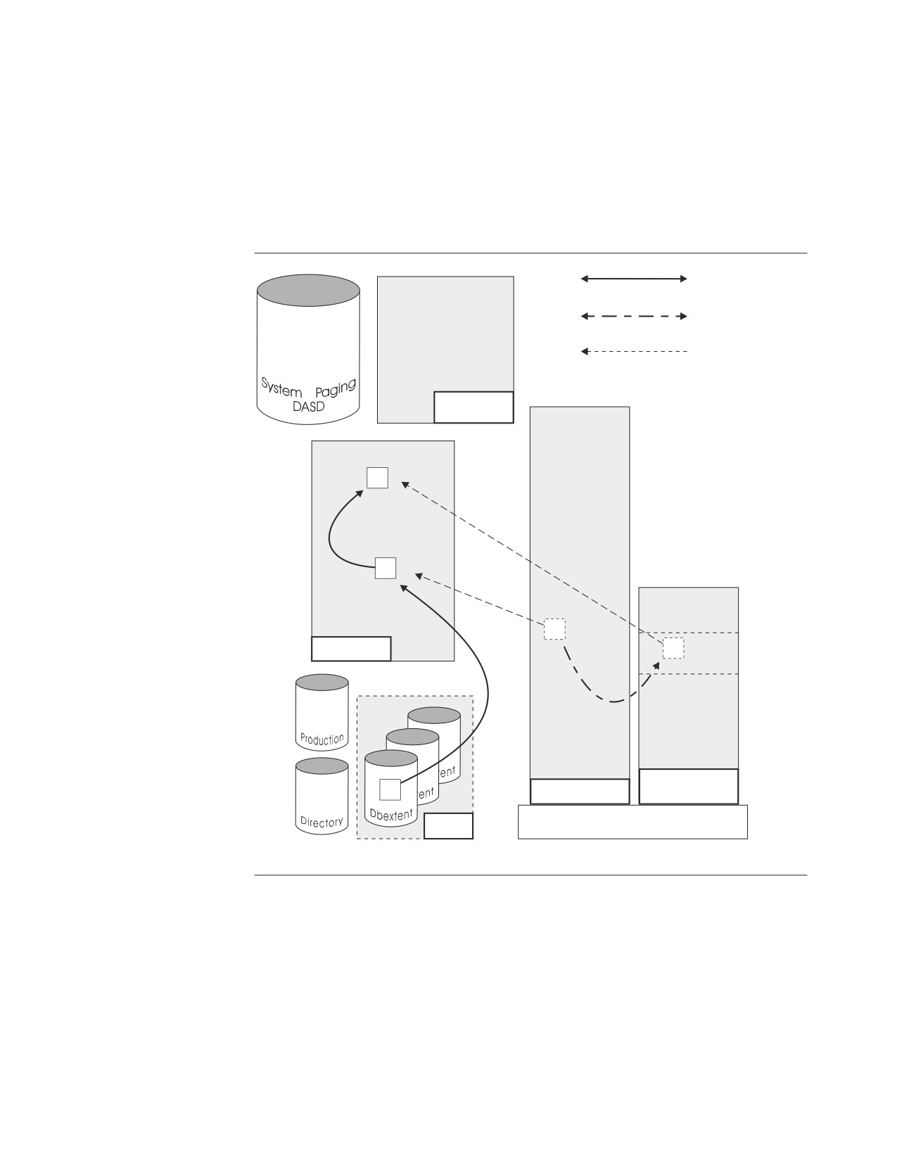
With Data Spaces Support on: If the database manager cannot find a page in its

buffer pools, it “retrieves” it from a data space and stores it in a free buffer in its

pool. When this happens, the operating system actually does most of the work. If

the page is already in main storage, the database manager can move it directly to

the buffer pool. If the page is in expanded storage or in DASD, the operating

system moves it into main storage, and then copies it into a buffer. If your

processor supports Enhanced Move Page for VM, pages are moved from expanded

storage directly into a buffer.

Physical Move

Virtual Move

Pointer From Virtual

to Physical Page

Expanded

Storage

Main Storage

Database

Data Space

Machine

Storage

Control Program

(CP)

Pool

Physical Storage

Virtual Storage

Figure 28. Page Movement with Data Spaces Support. The figure shows a page being read

into main storage from DASD and then into a buffer pool. The page will be in two places in

main storage until either the data space page is released or the database manager releases

the buffer page (refer to “Releasing Pages” on page 162).

This system has several advantages over the standard DASD I/O system, which

uses the IUCV *BLOCKIO service. In the latter, each page move must be explicitly

requested by the database manager, whereas here paging is done by the VM

paging system. This is faster and more efficient for several reasons, including:

v Shorter path length

v Asynchronous page fault processing

v Striping

Chapter 6. Data Spaces Support for VM/ESA

161

v Blocking and prefetching

v Dynamic storage size management

v More asynchronous writes.

Refer to “Deciding When to Use Data Spaces” on page 197 for a detailed

description of each advantage.

Releasing Pages

With Data Spaces Support off: When the database manager needs a buffer for

another page, it overwrites the “oldest” unmodified page in the pool with a new

page. This is referred to as releasing a page or stealing a buffer.

With Data Spaces Support on: When the database manager needs a buffer for

another page, it does so in the same way that it would with Data Spaces Support

off.

When the operating system needs main or expanded storage for itself or for other

virtual machines, it may release data space pages from main storage. Pages may

also be released at the request of the database manager. There are several

parameters you can use to control when the database manager will start releasing

pages and which pages it will choose (refer to “Managing Main and Expanded

Storage” on page 166).

Modifying Pages

With Data Spaces Support off: While a page is in the buffer pool, the database

manager may modify it. To ensure the integrity of your data, a modified page will

not be released until it has been written back to DASD. If the database manager

needs a buffer occupied by a modified page, it first writes the page to DASD, then

loads the buffer with a new page.

With Data Spaces Support on: Instead of writing the modified page to DASD,

the database manager moves it to a data space.

Once again, the operating system does most of the work. It takes the modified

page from the database manager and moves it into main or expanded storage.

If the operating system needs a main storage page that is occupied by that page, it

will move it to expanded storage or to DASD before it uses the main storage page.

Similarly, if it needs an expanded storage page that is occupied by a modified

page, it will move the modified page to DASD by way of main storage.

Checkpoints

At checkpoints, the database manager writes a summary status record to the log

and makes sure that all modified buffer pages and status information are written

to DASD. This ensures that you have a permanent record of your data on DASD.

With Data Spaces Support off: The database manager writes all the modified

pages that are still in the buffer pools to DASD. Until it is finished it cannot serve

any users.

With Data Spaces Support on: The database manager moves modified pages that

are still in the buffer pools to data spaces. It then directs the operating system to

save all the data space pages that were modified by the database manager to

DASD. Until the operating system is finished, the database manager is forced to

wait: it cannot serve any users until the checkpoint is complete.

162

Performance Tuning Handbook

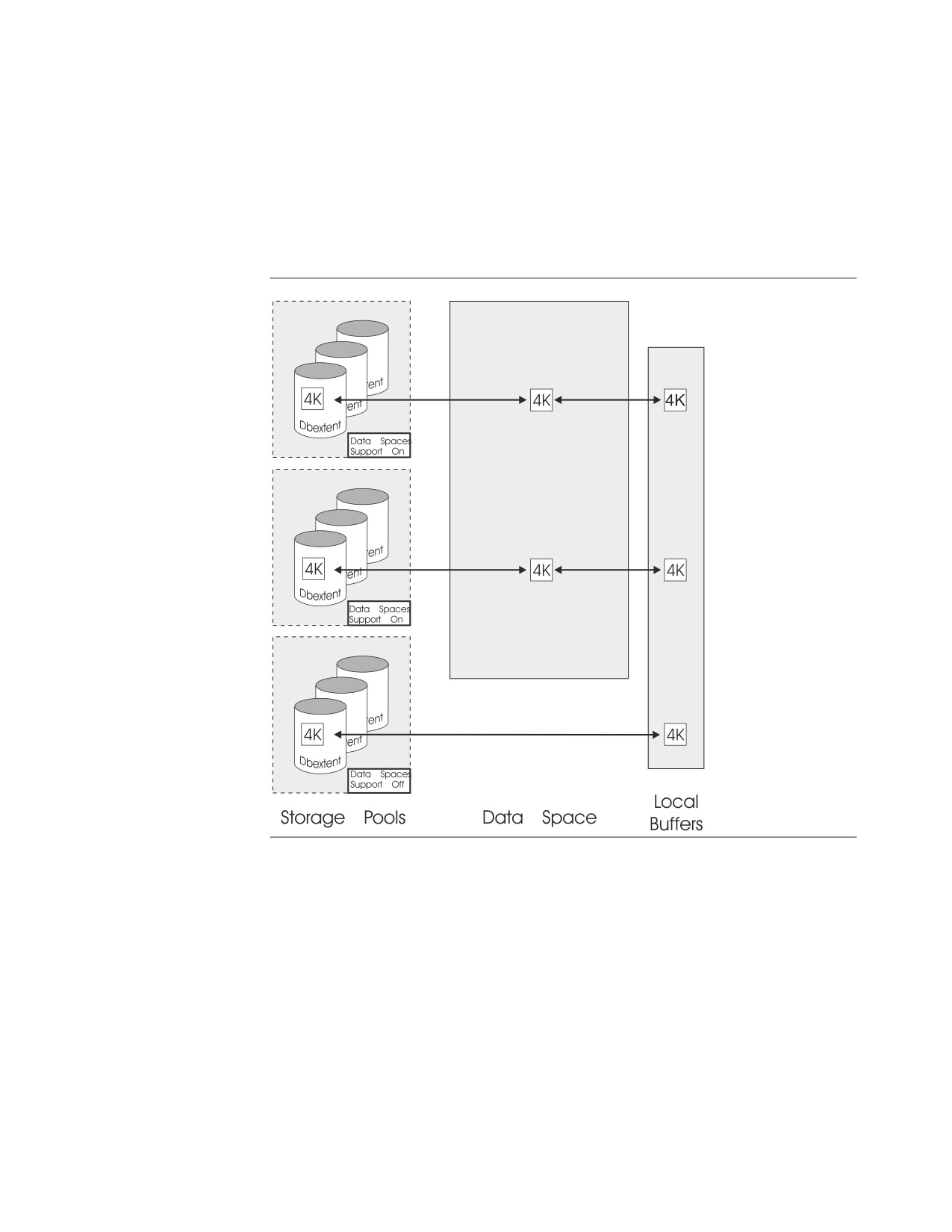
Storage Pools

Individual storage pools can be used with or without Data Spaces Support.

Note: A storage pool used only for internal dbspaces and which has a dbextent on

a virtual disk cannot be used with Data Spaces Support turned on for this

pool. For more information on virtual disk support for VM/ESA for internal

dbpsaces, refer to “Virtual Disk Support for VM/ESA for Internal Dbspaces”

on page 54.

Figure 29. Storage Pools with Data Spaces Support on and off

For a description of how to turn on Data Spaces Support, refer to “Specifying

Either Data Spaces Support or Standard DASD I/O” on page 189. For information

on when to use data spaces with storage pools, refer to “Storage Pool” on page

199.

Internal Dbspaces

Internal dbspaces can be used with or without Data Spaces Support.

Mapped Internal Dbspaces

Since internal dbspaces are assigned to a specific storage pool, you can turn Data

Spaces Support on and off for them by turning support on and off for that pool.

This type of Data Spaces Support is similar to the support for any other storage

Chapter 6. Data Spaces Support for VM/ESA

163

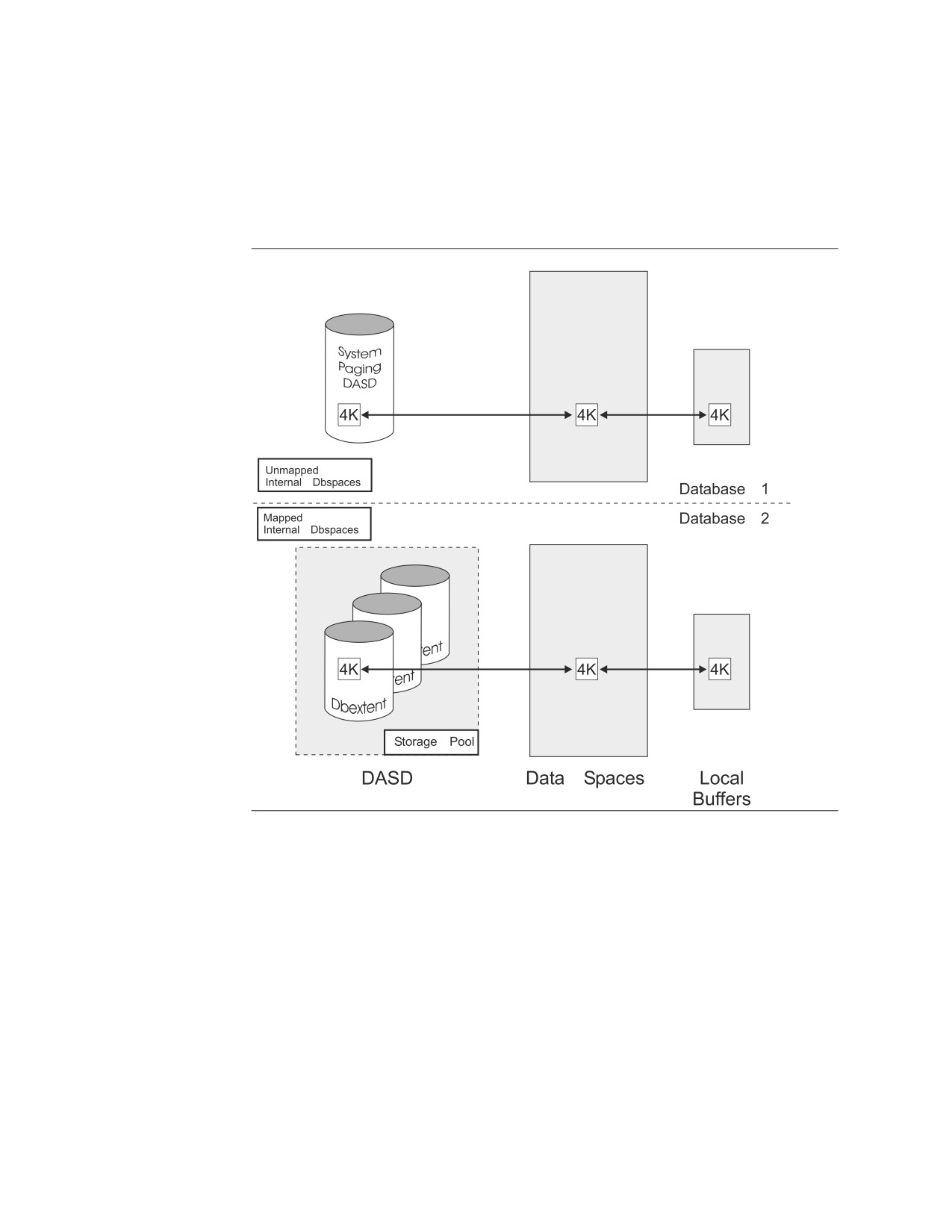
pool. Since the system assigns, or “maps” each data space page to a physical page

in a dbextent (contained in a storage pool), it is referred to as mapped support.

Unmapped Internal Dbspaces

VMDSS also supports unmapped internal dbspaces. Instead of mapping pages onto

dbextents, VM/ESA manages them as normal virtual storage paged to VM system

paging DASD (see Figure 30).

Figure 30. Unmapped and mapped internal dbspaces

The internal dbspaces are still assigned to a storage pool, but they do not use any

DASD in that pool. Rather they use system paging DASD. To make up for this,

you must allocate more DASD to system paging. Refer to “VM/ESA Paging

DASD” on page 173.

For a description of how to turn on Data Spaces Support for internal dbspaces,

refer to “Using Data Spaces with Internal Dbspaces” on page 192. For information

on when to use data spaces with internal dbspaces, refer to “Internal Dbspaces” on

page 199.

Directory

You can use the directory with Data Spaces Support either on or off.

164

Performance Tuning Handbook

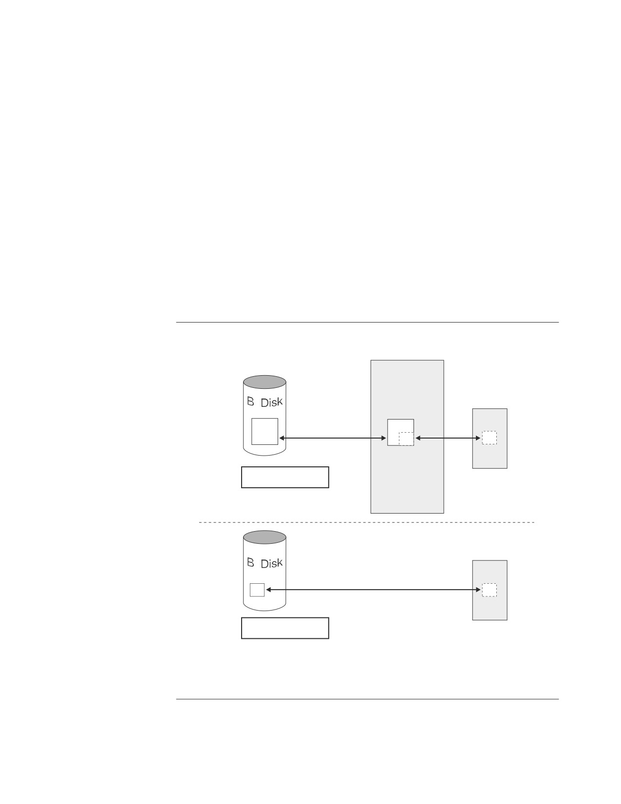
With Data Spaces Support off

The database manager stores directory data on the directory disk (B-disk) in

512-byte blocks and reads these blocks into the directory buffers from the B-disk as

necessary.

With Data Spaces Support on

The directory uses data spaces as a storage pool would. If the database manager

cannot find a block of directory data in the directory buffers, it gets the block from

a data space. If the directory block is not already in main storage, the operating

system locates the page on the B-disk that contains the directory block and copies

it into main storage (each 4KB page contains eight 512-byte directory blocks).

Any DASD accessed through a data space must have a 4KB block size. This means

that if you want to use the directory with Data Spaces Support, you must reblock

the directory minidisk from 512-byte blocks to 4KB pages.

For information on how to reblock and start Data Spaces Support for the directory,

refer to “Using Data Spaces with the Directory” on page 193. For information on

when to use Data Spaces Support with the directory, refer to “Directory” on page

200.

512

Directory Using

Data Spaces Support

Database 1

Database 2

512

Directory Not Using

Data Spaces Support

DASD

Data Space

B Disk

Buffers

Figure 31. The Database Directory with Data Spaces Support On and Off

Chapter 6. Data Spaces Support for VM/ESA

165

Managing Main and Expanded Storage

If unchecked, VMDSS may ask for large amounts of main and expanded storage

from the operating system. If it gets it, your database machine may be very fast

but other virtual machines in the system may perform poorly.

The operating system always maintains control of its main and expanded storage,

and will limit how much your database machine can use. If your machine tries to

use more storage than is available, the operating system will release some of your

pages (or pages from other virtual machines) from main or expanded storage to

make room for the new ones.

Instead of waiting for the operating system to release pages, you can instruct the

database manager to do so before your machine reaches its storage limits. Pages to

be released will be selected based on the parameters you set. You can also limit the

number of modified pages in main and expanded storage to improve checkpoint

processing.

The four primary parameters provided are:

v Target working storage size

v Working storage residency priority

v Checkpoint interval

v Save interval.

Target Working Storage Size Parameter

The target working storage size parameter controls the amount of main and

expanded storage that your database machine uses. When the amount of storage

reaches this target, the database manager will start to release certain data space

pages immediately after they have been copied into the buffer pools.

While you may exceed this target, the database manager will try to keep you at or

below it if possible. (Of course, you may never reach it if the operating system is

heavily loaded.)

You can set this parameter at start up time, or dynamically while the database

manager is running.

For information on how to change this parameter, refer to the DB2 Server for VSE

& VM Operation manual. For information on how to choose a value for it, refer to

“Choosing the Target Working Storage Size” on page 200.

Working Storage Residency Priorities

The database manager decides which data space pages to release based on the

working storage residency priority of each pool.

Priorities range from a value of 1 where all pages are released, to a value of 5

where none are. The priorities in between allow a page to be released depending

on whether your current working storage size is above or below your target, and

whether the page is an index or a data page.

For information on how to change storage priorities, refer to “Specifying Storage

Residence Priorities” on page 190. For information on how to choose a storage

priority, refer to “Choosing Storage Residence Priorities” on page 201.

The Checkpoint Interval

The checkpoint interval controls the duration between database checkpoints. At a

checkpoint, the database manager makes sure that all the modified pages in main

166

Performance Tuning Handbook

and expanded storage are written to DASD. (Refer to “Checkpoints” on page 162.)

If there are many modified pages, it can take a long time to complete the

checkpoint, and until it is complete the database manager cannot serve any users.

For information on how to change the checkpoint interval, refer to DB2 Server for

VSE & VM Operation. For information on how to choose a value for it, refer to

“Choosing the Checkpoint Interval” on page 203.

The Save Interval

To make checkpoint processing faster, you can limit the number of modified pages

in main and expanded storage by setting the save interval. When the number of

modified pages in a data space exceeds this parameter, the database manager

directs the operating system to save all the modified pages in that data space to

DASD. Unlike the save that occurs during checkpoint, the database manager can

continue to service users while this is being done.

For information on how to change the save interval, refer to the DB2 Server for VSE

& VM Operation manual. For information on how to choose a value for it, refer to

“Choosing the Save Interval” on page 203.

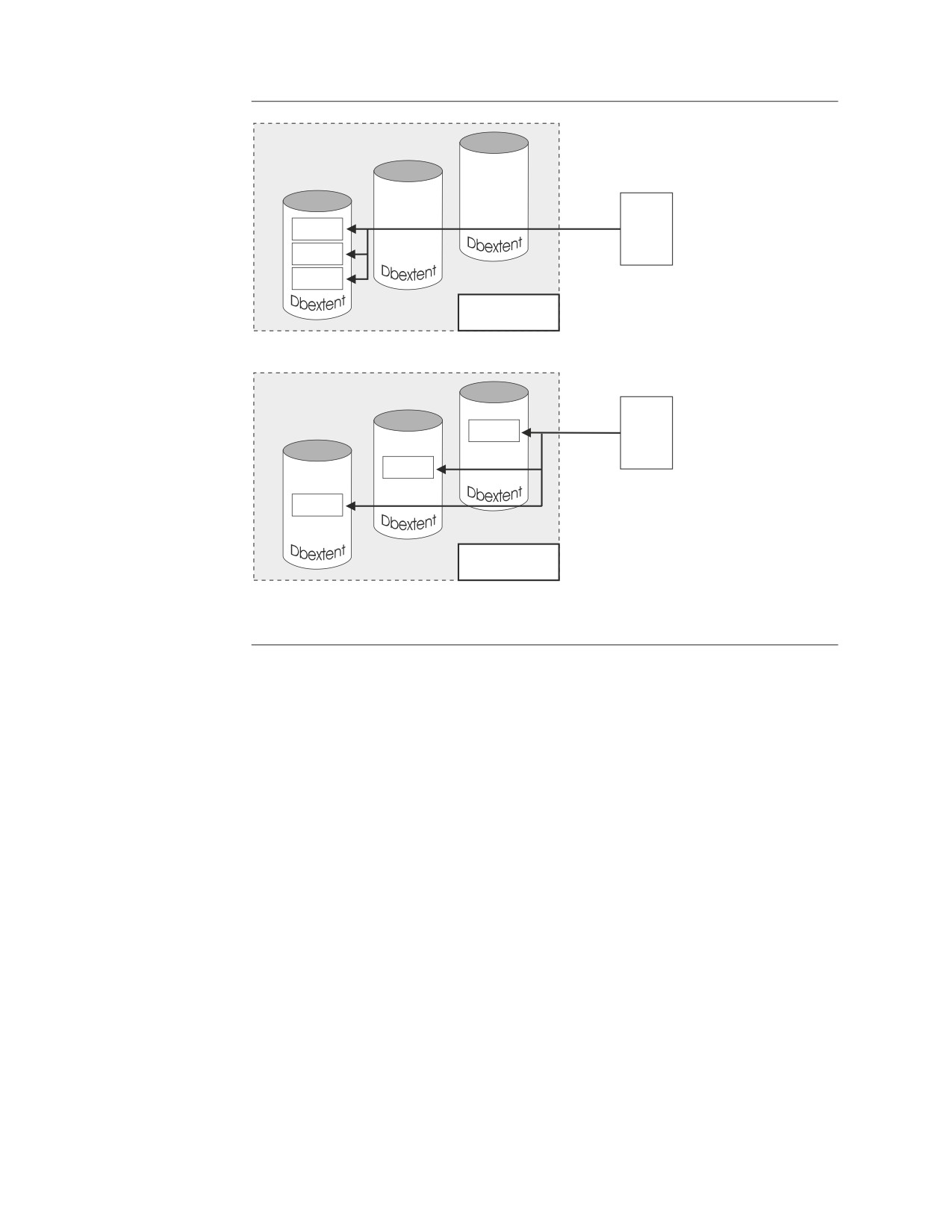
Striping

VMDSS will attempt to evenly distribute, or “stripe”, your data across all the

dbextents in a storage pool.

Chapter 6. Data Spaces Support for VM/ESA

167

01-16

4KB

Pages

17-32

33-48

Striping Off

33-48

4KB

Pages

17-32

01-16

Striping On

Storage Pools

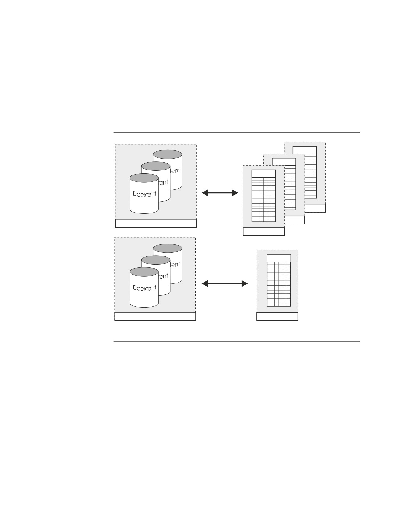
Figure 32. A storage pool with striping switched on and off. The figure shows 48 4KB pages

written to DASD with striping on and off.

With striping switched off

The database manager allocates pages in a storage pool in sequence, usually

allocating all the pages in one dbextent before using the next dbextent.

With striping switched on

The database manager allocates 16 pages in sequence on each dbextent in the

storage pool. The operating system can then read and write the pages to and from

DASD in parallel. This may significantly improve DASD performance, depending

on how you configure your controllers, channels, and DASD. The optimal

configuration would include several dbextents in the storage pool, each on a

separate channel, controller, and physical storage device.

For a description of how to use striping, refer to “Turning Striping On and Off” on

page 190. For information on how to decide when to use it, refer to “Using

Striping” on page 204.

Performance Counters

Several counters are available that can help you monitor the performance of the

DASD I/O systems. Each storage pool has its own set of four counters. There is

also a set of four counters for unmapped internal dbspaces, and a set for the

168

Performance Tuning Handbook

directory. These counters are different depending on whether a particular

component is using data spaces. (Unmapped internal dbspaces always use them.)

For more information refer to the DB2 Server for VSE & VM Operation manual. For

information on performance measurements in general, refer to Chapter 2,

“Measuring Performance,” on page 13.

Planning Structure by Storage Pool

You will need to design the structure of your database so that you can control it

effectively.

Table

Less Control

ace

Storage Pool

Dbspace

Table

More Control

Storage Pool

Dbspace

Storage Pools

Dbspaces

Figure 33. Planning for Critical Tables

We suggest in DB2 Server for VM System Administration that you have one table per

dbspace. Also, you may want to assign only one dbspace to each storage pool

because many of the VMDSS configuration options are grouped by storage pool:

for example, you can turn Data Spaces Support and striping on and off for a

particular storage pool, set residence priorities by storage pool, and display

counters by storage pool. By associating one table per storage pool, you can

determine how a specific table will use the VMDSS functions.

However, you should not do this for every table in your database. If you have

several tables that you always access together, place each one in a dbspace and

assign all the dbspaces to one storage pool. Only special tables where performance

and control are critical should have their own storage pool.

Chapter 6. Data Spaces Support for VM/ESA

169

Logical and Physical Mapping

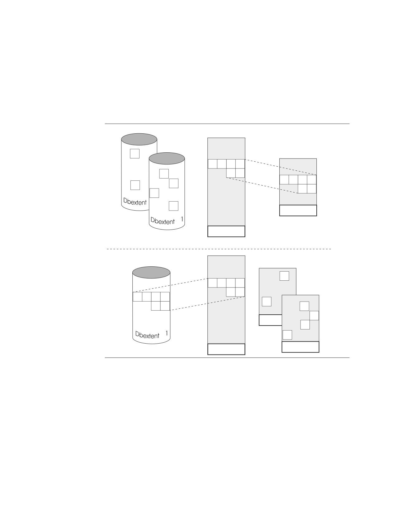
When you start the database manager, you can choose whether it will map data

space pages to physical pages, physical mapping, or virtual pages, logical mapping

(see below). The type of mapping you choose will apply to all the storage pools in

the database that are using Data Spaces Support.

For a description of how to set the type of mapping, refer to the DB2 Server for

VSE & VM Operation manual. For more information on how to choose one type,

refer to “Choosing Logical or Physical Mapping” on page 205.

Dbspace

Data

Space

Logical Mapping

Database

Physical Mapping

Dbspac

Dbspace

Data

Space

Figure 34. Logical and Physical Mapping

Logical Mapping

This associates (maps) each logical page in a dbspace to a data space page. Since

the logical pages are mapped onto a data space in the order they appear in the

dbspace, a contiguous set of pages in a data space will correspond to a contiguous

series of pages in a dbspace. This is the default and recommended mapping for

most applications.

Physical Mapping

This maps each physical page in a dbextent to a data space page. Since the

physical pages are mapped onto a data space in the order they appear on DASD, a

contiguous series of pages in a data space will correspond to a contiguous series in

physical storage.

170

Performance Tuning Handbook

VSE Guest Sharing

Although VMDSS does not support application servers running in VSE, VSE users

can access a VMDSS database in VM/ESA through guest sharing. The database

manager runs in one virtual machine, while the VSE users run under a VSE guest

system in another virtual machine. Since VMDSS only affects the database

manager, VSE guest sharing users will benefit from the same performance

improvements as VM users.

For more information on VSE guest sharing refer to the DB2 Server for VM Program

Directory.

Enabling Requirements

This section describes the operating system, virtual machines, software, virtual

storage, and hardware you need to enable and operate VMDSS.

Operating System Overview

To support all of VMDSS’s functions, you must:

v Enable it in VM/ESA Version 2 Release 3 (or later)

v Configure your database machine for Extended Configuration (XC) mode.

Operating in Non-XC Mode

If you are not operating in XC mode, you will not be able to use:

v Data Spaces Support for storage pools and the directory

v Unmapped internal dbspaces

v Working storage residency priorities

v Data space performance counters

v The target working storage size parameter

You will be able to use striping, and the storage pool performance counters for the

standard DASD I/O system.

Virtual Machine Overview

This section describes the virtual machines you need to enable and operate

VMDSS.

MAINT Machine

The MAINT machine, or its equivalent, already exists in all VM systems. It is

suggested that you use this machine to update the CP directory, although you can

use any machine with write access to the database minidisks and authority to

update the CP directory.

SQLMACH Database Machine

The database machine, usually called SQLMACH, owns the database minidisks. It

acts as an application server, either locally or remotely, within a TSAF collection or

SNA network. For more information, refer to DB2 Server for VM System

Administration.

To support all VMDSS’s functions, you must configure the database machine to

operate in XC mode. Refer to “Step 2: Update the CP Directory” on page 177.

You can configure the database machine to operate in ESA mode, but you will then

only be able to use a subset of VMDSS’s capabilities, as described in “Operating in

Non-XC Mode.”

Chapter 6. Data Spaces Support for VM/ESA

171

Software Requirements

To enable and operate VMDSS, you must first install DB2 Server for VM Version

Release 5.

Virtual Storage Requirements

This section describes the virtual storage the MAINT and SQLMACH machines

needed to use VMDSS.

MAINT Machine

You do not require any additional virtual storage for the MAINT machine.

SQLMACH Database Machine

You may need to add additional virtual storage to your database machine. To

calculate how much:

1. Add 41KB for additional VMDSS code.

2. Add 20KB if you are using data spaces

3. Add 2.5KB for each data space required. Refer to Appendix B, “Determining

Number of Data Spaces,” on page 211.

4. Add CUREXTNT X 16 bytes. CUREXTNT is the number of dbextents defined

during database generation.

5. Add MAXPOOLS X 8 bytes. MAXPOOLS is the maximum number of storage

pools that will ever be defined for a database.

6. Add MAXEXTNT X 8 bytes. MAXEXTNT is the maximum number of dbextents

that will ever be defined for a database.

7. Add MAXDBSPC X 8 bytes. MAXDBSPC is the maximum number of dbspaces

that will ever be defined for a database.

For example, consider a database generated with:

v CUREXTNT = 20

v MAXPOOLS = 256

v MAXEXTNT = 256

v MAXDBSPC = 10240

It is also currently using 10 data spaces for public and private dbspaces. The

database machine will use an additional 171KB of virtual storage:

41×1024 =

41,984

20×1024 =

20,480

2.5×10×1024 =

25,600

20×16 =

320

256×8 =

2,048

256×8 =

2,048

+ 10240×8 =

+ 81,920

174,400 =

174,400 = 170.40KB ∼ 171KB

Real Storage Requirements

While you do not require additional real storage (main or expanded storage) to use

VMDSS, any storage you add will be used by VMDSS to help improve the

performance of your database. Several facilities are included with VMDSS to help

you manage how much real storage you use. For more information refer to

“Managing Your Working Storage Size” on page 200.

172

Performance Tuning Handbook

DASD Storage Requirements

This section describes how much DASD space the VM system, the MAINT

machine, and the SQLMACH machine need in order to use VMDSS.

Fixed Block Storage Devices

The device number for a minidisk residing on an FBA DASD must start and end

on a 4K block boundary. The starting FBA block number and the ending FBA block

number +1 of the minidisk must be evenly divisible by 8. Refer to the MAPMDISK

information in the VM/ESA: CP Programming Services manual.

You can turn Data Spaces Support off for the Storage Pool residing on the FBA

device not on a 4K block boundary by updating the storage pool specification file.

To continue using an FBA device, use DDR or use the SQLCDBEX EXEC to copy

the extent to a new minidisk that is formatted on a 4K block boundary. Alternately,

you can move to a non-FBA device using the SQLCDBEX EXEC. Refer to the DB2

Server for VM System Administration for details on how to use the SQLCDBEX

EXEC.

VM/ESA Paging DASD

Before you can use separate internal dbspaces (unmapped), you may need to

allocate more DASD for VM system paging.

Attention: If VM runs out of system paging DASD, CP will abend if it does not

have sufficient spool DASD to accommodate the overflow.

To calculate the maximum number of additional cylinders you need for unmapped

internal dbspaces, divide the number of pages currently in all your internal

dbspaces by the conversion ratio for your type of DASD, listed in Table 11 and

round up to the nearest integer.

Table 11. Additional Paging Cylinders

DASD Type

3350

3375

3380

3390

9345

Conversion Ratio

120

150

180

150

(Blocks per Cylinder)

For example, if you are currently using 80 internal dbspaces of 1024 pages each for

your internal dbspaces, the calculation for 3380 DASD is as follows:

80*1024/150=546.133 cylinders

∼547

cylinders

Thus, you may need as many as 547 additional 3380 cylinders if you want to use

unmapped internal dbspaces. Remember, that the number you calculate will be the

maximum you will ever need. While you may actually use far fewer cylinders on a

day to day basis, you still need enough cylinders in either system paging DASD or

spool DASD to accommodate your peak requirements. If you cannot supply this

maximum value, you can still use mapped data spaces.

To assess your peak requirements, assign your internal dbspaces to their own

storage pool and use mapped internal dbspaces, refer to “Mapped Internal

Dbspaces” on page 192. You can then use the SHOW POOL operator command

(refer to DB2 Server for VSE & VM Operation) to see how many pages your

production system is really using for internal dbspaces. This will probably be

much lower than your maximum calculation. You can then allocate the number of

Chapter 6. Data Spaces Support for VM/ESA

173

pages the database manager is really using for the internal dbspace pool to system

paging DASD and start using unmapped internal dbspaces (refer to “Unmapped

Internal Dbspaces” on page 192).

Attention: The SHOW POOL command only displays the number of pages a pool

is currently using.

You must carefully monitor page usage over a relatively long period until you are

confident that the database manager will not use more pages than you will allocate

to system paging DASD. Also, remember to continue monitoring SHOW POOL

when you start using unmapped internal dbspaces in case your requirements

increase.

SQLMACH Database Machine

VMDSS requires a minimum amount of free space on the system minidisks.

System Disks: The system disks are the service and production minidisks or SFS

directories of the SQLMACH database machine. No additional DASD is required.

Database Disks: There are three types of database disks:

v Directory

v Log

v Data Extent.

While there is no change to the amount of DASD you require for your log or data

extent disks, the DASD you require for the directory disk may change depending

on how you use VMDSS.

If you use Data Spaces Support with the directory, you must move the directory

from a disk formatted with 512-byte blocks to one with 4KB blocks. Since 4KB

blocks use real DASD storage more efficiently than do 512-byte blocks, you do not

need as much real DASD storage.

To calculate the number of cylinders you need, multiply the number currently in

your directory disk by the conversion ratio for your type of DASD, listed in

Table 12 and round up to the nearest integer.

Table 12. Conversion from 512 byte to 4K byte blocks

DASD Type

3350

3375

3380

3390

9345

Conversion Ratio

0.85

0.63

0.57

0.51

0.52

For example, if you are currently using 34 cylinders of 3380 DASD for your

directory disk, the calculation is as follows:

34·0.57=19.38 cylinders

∼20

cylinders

Thus, you will only need a 20 cylinder disk after you move to 4KB pages.

You can also move the directory from a 4KB-block disk to a 512-byte-block disk. To

calculate how many cylinders you will then need, divide the number you need

when the directory is in 4KB blocks by the conversion and round up to the nearest

integer.

174

Performance Tuning Handbook

Hardware Requirements

To support all of VMDSS’s functions you must enable it in a ESA/390 processor

within the ES/9000^® family that supports VM/ESA in XC mode.

Before Enabling

This section describes what you need to read and what decisions you should make

before you enable VMDSS.

Program Directory for DB2 Server for VM

Study the DB2 Server for VM Program Directory which contains important service

information and special instructions.

Preventive Service Planning

Before you enable VMDSS, you should check whether there is any additional

Preventive Service Planning (PSP) information that you should know; check with

your IBM Support Center or use IBMLINK (ServiceLink).

This program release is maintained through the use of PTF tapes. An updated

Version or Release replaces the entire program code; a PTF tape only replaces the

changed portion of the program code.

For more information, refer to the DB2 Server for VM Program Directory.

Corrective Service

Follow the same corrective service procedures for VMDSS that you follow for DB2

Server for VM. For more information, refer to the DB2 Server for VM Program

Directory.

Enabling Options

You have several options when you enable VMDSS. Read the following to help

you evaluate which one you should use.

Using in a Production System

If you are using VMDSS on an existing production database, you may want to

carefully control which, if any, VMDSS functions you use. While the default

settings will turn all the functions on (with the exception of Data Spaces Support

for the directory), you can reset your operating parameters to turn everything off

before you restart your database.

With all the VMDSS functions off, you can ensure that your production system is

working as it was before you installed VMDSS. You can then selectively turn on

various components (you may need to stop and restart the database manager) and

monitor their effect.

Disabling Data Spaces Support

You can move your database manager to an operating system or hardware

platform that does not support VMDSS but does support DB2 Server for VM. You

may need to do this if you have a backup system that does not meet all of

VMDSS’s requirements.

Complete the steps listed in “Disabling VMDSS” on page 188; then, move your

database manager following your normal procedures.

Chapter 6. Data Spaces Support for VM/ESA

175

Resaving DB2 Server for VM in Saved Segments

If you previously stored the DB2 Server for VM DBSS component in a saved

segment, you can resave it after you enable VMDSS. Because VMDSS only affects

the DBSS component, and does not significantly increase its size (41KB), you can

use the default saved segment definition included with the base product. Refer to

“Step 10: Resave the DBSS Saved Segment” on page 181 for a description of how

to use VMSES/E and the ARISAVES EXEC to resave the DBSS component in a

saved segment.

Enabling

Perform the steps in this chapter to enable the VMDSS code onto the service and

production disks and to configure a database machine (SQLMACH) for VMDSS.

Pre-Enable Checklist

Before beginning, make sure that you have completed the following:

__ 1. Read Chapter 1, “Improving Performance.”

__ 2. Make sure that you have installed DB2 Server for VM Version 7 Release 5

with at least one 7.5.0 database available. You need this database to verify

the enabling of VMDSS.

__ 3. Decide whether you will configure the database machine for ESA or XC

mode.

__ 4. Make sure you have enough space on DASD to complete every step.

__ 5. Decide whether you will resave DB2 Server for VM components in saved

segments after you enable.

__ 6. Read the DB2 Server for VM Program Directory to check for any prerequisite

Program Temporary Fixes (PTFs) that need to be installed.

__ 7. See whether there is any additional Preventive Service Planning (PSP)

information that you should be aware of. Check with your IBM Support

Center or use IBMLink (ServiceLink).

Enable Checklist

Notes:

v Perform the steps in order.

v Mandatory steps are preceded by squares (u)

v Conditional steps are preceded by circles (V)

v Page references appear in parentheses.

1. u Log onto the MAINT Machine ( 177)

2. V Update the CP Directory ( 177)

3. u Log off the MAINT Machine ( 178)

4. u Log onto the SQLMACH Machine ( 178)

5. u Archive your Database ( 178)

6. u Activate VMDSS ( 179)

7. u Log off the SQLMACH Machine ( 179)

8. u Log onto the DB2 for VM Installation User ID (5697F42X) (

179)

9. u Link-Edit the Load Library ( 180)

10. V Resave the DBSS Saved Segment ( 181)

a. V Prepare to Build the DB2 for VM Segments ( 181)

b. V Build the DB2 for VM Segments ( 182)

c. V Create a Bootstrap Package ( 182)

176

Performance Tuning Handbook

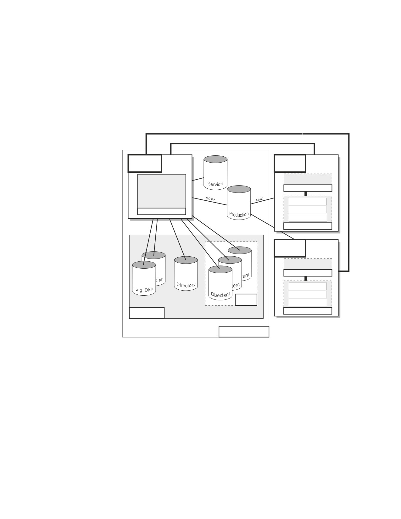
d. V Restart the Application Server ( 184)

11. u Log off the DB2 for VM Installation User ID ( 184)

12. u Log onto the SQLMACH Machine ( 184)

13. V Verify the Installation ( 184)

a. V Verify non-XC Mode Installation ( 184)

b. V Verify XC Mode Installation ( 186)

14. V Optional System Activities ( 187)

Communication Link (IUCV or APPC/VM)

Database

User

Machine

Application Requester

Interactive SQL

Preprocessors

Database Manager

DBS Utility

Applications

User

Machine

Application Requester

Interactive SQL

Preprocessors

Storage

Pool

DBS Utility

Applications

Database

Application Server

Figure 35. Typical DB2 Server for VM System Setup

Backing Up, Configuring and Enabling Your Database Machine

Perform the following steps to:

v ensure that you have a current backup of your database

v update your database machine for VMDSS

v enable the VMDSS code.

Step 1: Log onto the MAINT Machine

Log onto the MAINT machine.

Step 2: Update the CP Directory

Skip this step if you plan to configure your database machine for ESA mode or if

you already updated the CP directory for XC mode when you planned the initial

install of DB2 Server for VM.

Chapter 6. Data Spaces Support for VM/ESA

177

To use all the VMDSS functions, you must add the statements shown in Figure 36

to the CP directory entry for the database machine.

MACHINE XC

XCONFIG ACCESSLIST ALSIZE 1022

XCONFIG ADDRSPACE MAXNUMBER 1022 TOTSIZE 2044G

Figure 36. Additional Directory Control Statements for the Database Machine

Statement 1: MACHINE XC

Specifies that the database machine will simulate the VM/ESA XC

architecture.

Statement 2: XCONFIG ACCESSLIST ALSIZE 1022

Statement 3: XCONFIG ADDRSPACE MAXNUMBER 1022 TOTSIZE 2044G

The ALSIZE and MAXNUMBER parameters in these two statements

specify the maximum number of data spaces that the database machine

can create and have existing concurrently. For VMDSS, ALSIZE and

MAXNUMBER should be set to the same value.

The value in this example, 1022, is the upper limit for these parameters.

Since there is no cost in setting this value high, the value 1022 should be

acceptable for most applications. To precisely calculate the maximum

number of data spaces that your database machine will use, refer to

Appendix B, “Determining Number of Data Spaces,” on page 211.

TOTSIZE specifies the maximum total size, in bytes, of all the data spaces

that the database machine can create and have existing concurrently.

Since each data space is 2GB, your maximum total size for 1022 data

spaces will be 2044GB. For a description of how to precisely calculate the

maximum total size of the data spaces for your database, refer to

Appendix B, “Determining Number of Data Spaces,” on page 211.

For more information on the MACHINE and XCONFIG directory statements, refer

to the VM/ESA: Planning and Administration.

When you have finished adding the CP directory control statements for the

database machine, update the CP directory using your current operating

procedures.

Step 3: Log off the MAINT Machine

Log off the MAINT machine.

Step 4: Log onto the SQLMACH Machine

Log onto the database machine (SQLMACH). Refer to “SQLMACH Database

Machine” on page 174 for information on this virtual machine.

Step 5: Archive your Database

While installing VMDSS does not affect the data in your database, it is always

good practice to archive your database before installing new code or applying

service. If you do not archive your database on a regular basis, LOGMODE=Y or N

(Y is the default), skip this step.

178

Performance Tuning Handbook

If your application server is currently running with LOGMODE=L or A, you can

perform a user archive or a database archive. To create a database archive, type:

SQLEND ARCHIVE

As with any archive, the database manager requests that you mount the required

tape volume to contain the database archive (or log archive, if LOGMODE=L, and

you are not archiving the log to disk). The database manager then creates the

archive. When the database manager prompts you to mount and ready the archive

volume, you should respond with the virtual device number. Unless you have

issued your own CMS FILEDEF command before starting the database manager,

the virtual device number for database archives is 181. The virtual device number

for log archives is 183.

For more information on the SQLEND command, or information on user archives,

refer to DB2 Server for VM System Administration.

Step 6: Activate VMDSS

To enable (or remove) the VMDSS code, perform the following steps on the

database machine user ID. These steps must be performed on every database

machine on which you wish to use VMDSS.

1. Be sure you are logged on to the database machine (SQLMACH).

2. Stop the application server using your normal operating procedures.

3. Ensure that the database machine production disk and service disk are linked

in write mode. If not, enter:

LINK machid 195 195 W

LINK machid 193 193 W

4. Access the production disk with file mode Q and the service disk with file

mode V.

ACCESS 195 Q

ACCESS 193 V

If you are using SFS directories instead of minidisks, access them with file

modes Q and V.

5. Run the ARISDBMA EXEC to identify whether you want DSS code enabled on

your production disk. Its syntax is:

►► ARISDBMA DSS( Y

)

►◄

Specify the following parameters:

Enable the DSS code. This is the default.

N Disable the DSS code.

For example, to identify that you want to enable or disable the DSS code, type:

ARISDBMA DSS(Y)

ARISDBMA DSS(N)

Step 7: Log off the SQLMACH Machine

Log off the database machine.

Step 8: Log onto the DB2 for VM Installation User ID (5697F42X)

Log onto the DB2 Server for VM Installation user ID, 5697F42X.

Chapter 6. Data Spaces Support for VM/ESA

179

Step 9: Link-Edit the Load Library

Rebuild the database manager with VMDSS by link-editing the DBSS component

in the ARISQLLD loadlib.

Make sure you have read access to the VMSES/E code (MAINT 5E5 disk) and

read/write access to the Software Inventory disk (MAINT 51D) or SFS

directory.

Establish the access order.

vmfsetup 5697F42X {DB2VM|DB2VMSFS}

5697F42X is the PPF that was shipped with the product. If you have your own

PPF override, substitute that name for 5697F42X shown in this command. You

also need to substitute your PPF name in the VMSES/E commands in any

subsequent steps.

Use DB2VM for installing on minidisks or DB2VMSFS for installing in Shared File

System directories.

Rebuild DB2 Server for VM DBSS member or component in the ARISQLLD

LOADLIB. You must do both steps 3a and 3b.

a. Rebuild the ARISQLLD LOADLIB.

vmfbld ppf 5697F42X {DB2VM | DB2VMSFS} ARIBLLLD ARISQLDS (all

vmfview build

Use DB2VM for installing on minidisks or DB2VMSFS for installing in Shared

File System directories.

ARIBLLLD is the name of the VMSES/E build list used to build the

ARISQLLD LOADLIB.

Review the build message log ($VMFBLD $MSGLOG). If necessary, correct

any problems before you continue. Use the F2 key, ALL, to review all of the

messages.

Note: The following message is normal if you are NOT running DB2 Server

for VM with the DB2 Data Spaces Support:

VMFLLB2074I Part xxxxxxx TXT in object ARISQLDS

in build list ARIBLLLD

EXEC will be ignored

b. Build the related files.

vmfbld ppf 5697F42X {DB2VM | DB2VMSFS} (serviced

vmfview build

Use DB2VM for installing on minidisks or DB2VMSFS for installing in Shared

File System directories.

Review the build message log ($VMFBLD $MSGLOG). If necessary, correct

any problems before you continue.

Link and access the database machine user ID production and service disks or

SFS directories.

link SQLMACH 195 295 MR

acc 295 l

link SQLMACH 193 293 MR

acc 293 m

You will be prompted for the password to the disks.

Substitute your minidisk addresses, if different.

Substitute in the appropriate SFS directory names.

180

Performance Tuning Handbook

DB2 Server for VSE. Operations Guide / Handbooks (2004-2007) - page 31