Content      ..     22      23      24     

PowerWorld Simulator version 11. Manual - page 24

Tutorials

· This opens the Bus Field Options dialog (shown below); select the field Bus Voltage to add in the selected position

and click OK.

· The parameter and position are displayed as highlighted in the Insert New Fields dialog. Click OK. Note that the

specified bus field has been added to the oneline diagram.

· Repeat this procedure for the other two buses. If necessary, you may move fields manually with the mouse.

Fields can also be inserted using the Insert > Field option from the main menu or by using the Insert Field buttons on

the Insert Toolbar.

Next, we will insert fields showing the power flow at each end of the transmission line.

·

Select Insert > Field > Line Field or click the Line Field button on the Insert toolbar.

Line fields show information about trans mission lines and transformers. For line fields, flow is always specified at an

end of the transmission line or transformer. The end is normally determined automatically by the insertion point.

·

Left-click near both bus 1 and the transmission line between buses 1 and 2 in the location you want the power

flow text to appear. The Line Field Options dialog (shown below) opens automatically.

·

The Near Bus and Far Bus fields should show 1 and 2 respectively. If they do not, enter the correct values.

·

Select AC Line MW Flow then click OK. The field is displayed on the oneline in the location you specified. Note

that the field can be moved and formatted as previously discussed.

·

Select Insert > Field > Line Field or click the Line Field button on the Insert toolbar.

·

Left-click near both bus 2 and the transmission line between buses 1 and 2 in the location you want the power

flow text to appear. The Line Field Options dialog (shown below) opens automatically.

·

Now the Near Bus and Far Bus fields should show 2 and 1 respectively. If they do not, enter the correct values.

·

Select AC Line MW Flow then click OK.

·

Repeat the procedure to insert AC Line Mvar Flow fields for the two locations.

923

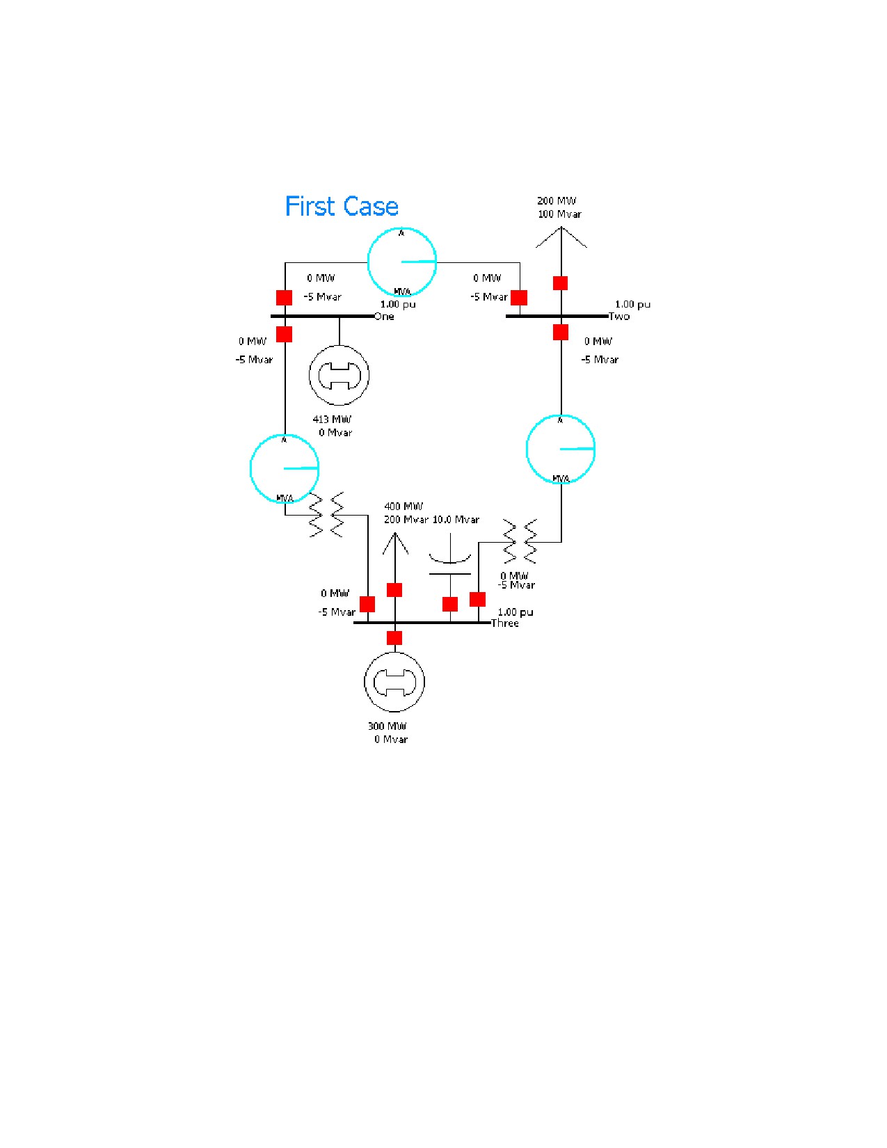
We also desire to monitor the MW and Mvar flows on the lines joining buses 1 and 3 and buses 2 and 3 via the

transformers. The same commands are used as those used to insert fields for the transmission line.

·

Repeat the above steps to insert AC Line MW (and Mvar ) Flow fields on the lines joining buses 1 and 3 and

buses 2 and 3 via the transformers.

·

At this point, your first oneline diagram should resemble the one shown below.

·

Save the case.

924

Tutorials

Tutorial: Solving the Case Page 12 of 13

To solve a case, you must be in run mode:

·

Click on Run Mode button on the Pr ogram Toolbar. Note that, if the case has validation errors, a warning will

appear. You will need to rectify the problems before you can enter Run Mode.

·

Select Simulation > Play to begin the simulation (or press the Play

button on the Run Mode toolbar).

Alternatively, to perform a single Power Flow Solution, click the Single Solution button on the Program Toolbar.

Your case should look similar to the case shown below. If it does, congratulations! You have completed building

your first case.

Try clicking on the load circuit breaker to toggle the load’s status. A solid red circuit breaker indicates that it is closed,

a hollow green box indicates it is open. While the simulation is running, click on the circuit breakers and note the

nearly instantaneous change in system flows. If the Log window is visible, you will get a "backstage" view of what

Simulator is doing. Feel free to close the log. To re-open the log, click the Log

button on the Program Toolbar.

With the load circuit breaker closed, open the circuit breaker between bus 3 and its connected generator. Now open

any of the transmission line or transformer circuit breakers.

Congratulations, you’ve just blacked-out your case!

925

Tutorial: Adding a New Area

Page 13 of 13

Next, we will create a second operating area for the case. Large interconnected systems usually have a number of

control areas, with each control area responsible for the operation of a particular part of the system. Often, a single

control area corresponds to a single owner (such as an investor-owned utility), but it is not unusual for a single control

area to have more than one owner. Control areas are connected to neighboring areas through tie lines. A tie line is a

transmission line that has one end in one control area and the other end in another. The total amount of power flowing

out of a control area is the algebraic sum of the power flowing out on all the area’s tie lines. Each control area is

responsible for procuring enough power to meet its own load plus losses. The control area can get this power either

by generating it itself, or by buying it from another area. This ability to buy and sell power (i.e., power transactions) is

one of the principal advantages of interconnected operation.

To create another control area:

·

Change to Edit Mode . Right click on bus 3 and select Bus Information Dialog from the dropdown menu.

·

Entering a number for an area that does not already exist automatically creates a new area. Enter ‘2’ in the Area

Number field. Enter ‘TWO’ in the Area Name field. Click OK.

·

To verify that the case now has two areas, select Case Information > Case Summary from the main menu. The

Case Information Displays allow you to view the entire case using non-graphical displays. The Case Summary

dialog (shown below) shows the number of buses, generators, lines/transformers, and control areas in the case.

You cannot modify any of these values.

Now we will make sure that both of the control areas are initially set as being on automatic generation control (AGC).

AGC insures that the generation in the area is equal to the load plus losses plus and scheduled transactions.

·

Select Case Information > Areas . The Area display (pictured below) provides a convenient summary of all the

control areas in the case. Similar displays exist for buses, generators, lines/transformers, etc.

926

Tutorials

·

Right-click anywhere on the record for the first area and select the Show Dialog option. The Area Display Dialog

is shown (as below).

·

Change the Area Name to ‘ONE’ and set the AGC Status under Area Control Options to Economic Dispatch

Control. Select SAVE to save this information.

·

Next click on the up arrow next to the right of the Area Number field. This displays the Area Record dialog for the

next area. Set the AGC Status to Economic Dispatch Control, and select OK to save your changes and close

the dialog.

·

Note the AGC Status field in the Area Records Display now shows ED in the AGC Status fields. Close the Area

Records display.

927

Tutorials

Tutorial: Loading an Existing Power Flow File Page 2 of 15

Once Simulator has been started, set Simulator to Edit Mode by clicking on the Edit Mode button on the Program

Toolbar. Select the File > Open Case from the main menu, or select the Open Case

button on the File Toolbar.

An Open dialog box will appear on the screen. To select a power flow file, click on the Type of File field in the lower

left hand corner of the dialog box. A list of file formats will appear. Choose the appropriate format, and the available

files of the type selected will appear in the box above Type of File . Choose the desired f ile from the list of available

files and select OK. In this example, we will be building a oneline for the 3990 bus MAIN 1998 summer case saved in

PTI version 23 format as mdb98s.raw. When prompted to create a oneline, select ‘yes’. Your display should

immediately turn white. This shows the blank background upon which you will be drawing the oneline diagram for your

case. Onelines are used in power system analysis to represent the actual three-phase power system using a single

line to represent each three phase device. The information from the power flow file is now accessible to Simulator.

929

Tutorial: Case Information Displays Page 3 of 15

Simulator presents many different Case Information Displays to provide a text-based view of the case. For example,

to view or modify the description of the case, select Case Information > Case Description from the main menu. The

Case Description Dialog should appear, showng the text description of the power flow case. In PowerWorld, this

text description may be arbitrarily long.

You can also obtain a case summary by selecting Case Information > Case Summary from the main menu. The

summary dialog will appear. It provides a summary of the case and of the total case load and generation. None of the

fields in this dialog can be changed, as they are intended for informational purposes only.

The Area/Zone Filters information display is another important article. The Area/Zone/Owner Filters feature restricts

the contents of other case information displays to certain areas or zones. This is particularly useful for large cases.

Open the Area/Zone Filters display by selecting Case Information > Area/Zone Filters from the main menu, or use

the Area/Zone/Owner Filters button on the Options/Info Toolbar. As with all Case Information Displays, you can click

on a column heading to sort the list on a particular field; click on that same column heading again to reverse the sort

order. To change a particular area’s area/zone filter status, simply left-click on the area’s area/zone filter status field.

To change the filter status for all areas in the case, right-click on the display to bring up its local menu (all case

information displays have a local menu), and select either Toggle All Yes or Toggle All No. For our example, set all

areas to ‘no’ except WUMS.

Another important text-based display is the Power Flow List. The power flow list shows the complete power flow

information for all areas whose area/zone filter is set to ‘yes’. To display the power flow list, select Case Information

> Power Flow List. The power flow list has other options that can be accessed by right-clicking anywhere on the list.

If you wish to view more details about a particular device, you can do so by holding down the Ctrl key and left-clicking

on the device. To move through the list of buses, you can use the arrow keys or the scroll bar. If you are viewing a

particular bus and you wish to view a bus connected to it, double-click on the line connecting the two buses to view the

flows at the other bus. Note that some of the transmission lines have a circuit identifier of ‘99’. Whenever a ‘99’ is

used for an identifier, it usually means that the transmission line is an equivalent line.

A shorter version of the power flow list can often be more useful. Such a display is offered by the Quick Power Flow

List. The Quick Power Flow List is similar to the power flow list except that it shows flows at individual buses or a set

of buses, regardless of area/zone filter settings. You can view flows at any bus in the case. To display the quick

power flow list, select Case Information > Quick Power Flow List from the main menu, or press the Quick Power

Flow List

button on the Options/Info Toolbar. Identify the buses of interest In the Bus Number field by entering

the number of either a single bus, a set of buses separated by commas, or a range of buses specified using a hyphen.

Again you can double-click to move to a desired bus, or choose Show Object Dialog from the display’s local menu to

see the information dialog for any object.

930

Tutorials

Tutorial: Entering a Bus Page 6 of 15

The most important component of the power system model is the bus. Buses are used to represent junction points in

the power system where a number of devices connect together. To build a oneline diagram, you draw the buses,

attach devices such as generators and loads to the buses, and connect the buses together with transmission lines and

transformers.

To begin entering devices onto the blank oneline, you must first switch to Edit Mode. If you are not already in Edit

Mode, switch back to Edit Mode now. Show the Quick Power Flow List and move it towards the bottom of the screen.

Show bus 39820 by typing that number in the Bus Number field. Select Insert > Bus from the main menu, or click

the Bus

button the Insert Toolbar. Click on the oneline towards the top center to define the point at which the

new bus will be added. The Bus Information Dialog will appear. In the Bus Number field enter 39820. Select Find

by Number to view the bus information. You should see the information appear in the Bus dialog fields that

corresponds with the MAIN power flow case. Select OK to place the bus. The bus should now appear on your

screen.

If it has not already been done for you automatically, add a bus field identifying the new bus’ number immediately to

the left of the new bus. To do this, click on or to the left of the display object that represents bus 39820 and select

Insert > Field, Bus from the main menu. Alternatively, click the Bus Field

button on the Insert Toolbar. The

Bus Field Options Dialog will appear for you to fill out. Designate the type of field as Bus Number and close the dialog.

Simulator will add a text object showing the bus number at the point where you had clicked.

Repeat this procedure to place buses 39881 and 39821 on the oneline, along with their bus numbers.

933

Tutorial: Automatic Line Insertion Page 7 of 15

Transmission lines between buses can be inserted manually by choosing Insert > Transmission Line from the main

menu or pressing the Transmission Line

button on the Insert Toolbar, clicking on the beginning bus, and

tracing a line to the ending bus. Vertices may be defined along the way by clicking the mouse on the diagram where

vertices should appear. However when creating a case from an existing power flow file, you also have the option to

insert transmission line display objects automatically. To do this, select Insert > Auto Insert > Lines from the main

menu in Edit Mode. Accept the default options and click OK. The lines joining the visible buses on the display are

automatically added, along with circuit breakers and pie charts, provided those options are set. Simulator will draw

only transmission lines that link buses that have already been drawn on the oneline diagram. If you add another bus

to the diagram, you can again auto-insert lines, and Simulator will only insert lines that are not already present on the

display.

934

Tutorials

Tutorial: Simulating the Case Page 10 of 15

Once you have constructed a oneline diagram showing the area of interest, you can simulate the case. Simulator

cannot only show the magnitude and direction of flows on transmission lines, but it can also animate them. To

configure the animated flows, switch to Edit Mode and choose Options > Oneline Display from the main menu.

Select the Animated Flows Tab of the resulting dialog box. Check the Show Animated Flows check box to enable

the animated flows at run time. This dialog box also allows you to change the size, density, and fill color of the

animated flows for easier visualization. At this point, just click OK. Next, save your case by selecting File > Save from

the main menu or by pressing the Save

button on the File Toolbar. If you have not already saved the case, a

Save As dialog will prompt you to select a name. Both the oneline diagram and the case will use this name.

To perform the simulation, switch to Run Mode and select Simulation > Play or Simulation > Restart from the main

menu. You should now see Simulator modeling the 3990-bus case.

937

Tutorial: OPF Three Bus Example

Page 2 of 6

For this tutorial, we will start with a provided three-bus case (B3LP) found in the PowerWorld\Simulator\Sample Cases

directory. Bus 1 is the system slack bus. All buses are connected via 0.1 pu reactance lines, each with a 100 MVA

limit. There is a single 180 MW load at bus 3. The generator marginal costs are:

-

Bus 1: 10

$/MWhr; Range = 0 to 400 MW

-

Bus 2: 12

$/MWhr; Range = 0 to 400 MW

-

Bus 3: 20

$/MWhr; Range = 0 to 400 MW

To begin:

· Load B3LP case.

· Verify the above system specifications by right clicking on each line, bus, and generator and selecting its respective

Line/Bus/Generator Information Dialog from the drop down menu.

· Select Run Mode .

· To be included in the OPF, all required area AGC status fields must be selected to OPF. To set area AGC to OPF:

Select LP OPF > OPF Areas . The OPF Area Records display automatically opens. Verify the AGC Status field is

selected to OPF. If it is not, double click on the field to change its value. Close the OPF Area Records display.

· Select LP OPF > Primal LP to solve the case. Note: line limits are not initially enforced.

Your display should look similar to the following:

B3LP Solved Using LP OPF > Primal LP

Note the line from Bus 1 to Bus 3 is overloaded and that all buses have the same marginal cost.

944

Tutorials

Tutorial: OPF Line Limit Enforcement

Page 3 of 6

·

Select LP/OPF > OPF Areas .

The Branch MVA column specifies whether or not the MVA limits should be enforced for transmission lines and

transformers that have at least one terminal in this area. For a transmission line or transformer to be included in the

OPF constraints, Line/Transformer constraints must not be disabled on the OPF Options Dialog, and the individual

line/transformer must be enabled for enforcement on the OPF Line/Transformer MVA Constraints display.

·

Double click on the Branch MVA field to change the value to YES. Close the OPF Area display

·

Select LP/OPF > Options .

·

The LP OPF Dialog opens automatically. Select the Constraint Options tab then click Disable

Line/Transformer MVA Limit Enforcement to remove the checkmark.

·

Click Solve LP OPF then click OK.

B3LP Solved with Line Limit Enforcement Enabled

The LP OPF re-dispatches to remove the line limit violation. Bus marginal costs have changed from the initial

example. The new bus marginal cost at Bus 3 is 14

$/MWh. To verify this:

·

Increase the load at Bus 3 by 1 MW. Right click on the load, enter "181.0" in the Constant Power / MW Value

field in the Load Options dialog. Click OK.

·

Select LP OPF > Primal LP.

The Total Cost increased to 1935

$/hr from the previous value of 1921

$/hr, a difference of 14

$/hr when Bus 3 load

was increased by 1 MW.

945

Tutorial: OPF LMP Explanation

Page 4 of 6

Explanation of Bus 3 LMP = 14

$/MWh (from previous page):

B3LP Solved with Line Limit Enforcement Enabled

All lines have equal impedance. Power flow in a simple network distributes inversely to impedance of the path.

·

For Bus 1 to supply 1 MW to Bus 3, 2/3 MW will take the direct path from 1 to 3, while 1/3 MW will take the path

from 1 to 2 to 3.

·

Likewise, for bus 2 to supply 1 MW to Bus 3, 2/3 will go from 2 to 3, while 1/3 will go from 2 to 1 to 3.

·

To supply one additional MW to Bus 3, we need the change in power of generator 1 (Pg1) plus the change in

power of generator 2 to equal 1 MW.

Pg1 + Pg2 = 1 MW

·

With the line from 1 to 3 limited, no additional power flows are allowed on it.

(2/3)Pg1 + (1/3)Pg2 = 0

·

Solving the above system of equations results in:

Pg1 = -1 MW and Pg2 = 2 MW

Dcost = S(DPg*LMP) = [(-1 MW)*(10.00

$/MWh) + (2 MW)*(12.00

$MW/h)] = 14.00

$/hr

946

Tutorial: OPF Unenforceable Constraints

Page 6 of 6

Next we will consider a case with unenforceable constraints. To begin, increase the load at Bus 3 to 250 MW then run

the LP OPF again:

·

Right-click on the load at Bus 3. Enter 250 in the Constant Power / MW Value field.

·

Select LP OPF > Primal LP.

B3LP with Bus 3 Generator Carrying Load

Note that the transmission lines connecting Bus 3 to the other buses are both at their respective MVA limit and that the

generator at Bus 3 is supplying the load in excess of the transmission line limits. Next we will open the generator at

Bus 3 thereby inserting an unenforceable constraint:

·

Left-click on the red breaker symbol connecting the generator to Bus 3 to open the breaker.

·

Select LP OPF > Primal LP.

B3LP Solved with Unenforceable Constraints

Both constraints cannot be enforced. If a constraint cannot be enforced due to insufficient controls, the slack variable

associated with enforcing that constraint can not be removed from the LP basis.

948

Tutorials

Note the new LMP value for bus 3 exceeds 1000

$/MWh. Marginal cost depends on the arbitrary cost of the slack

variable. This value is specified in the Marginal Violation Cost field of the LP OPF > Options dialog. See OPF

Options dialog for more details.

Additional Example

To see another OPF example select PowerWorld Simulator Add-on Tools > Optimal Power Flow (OPF) >

Examples from the table of contents in the on-line help file.

Contingency Analysis

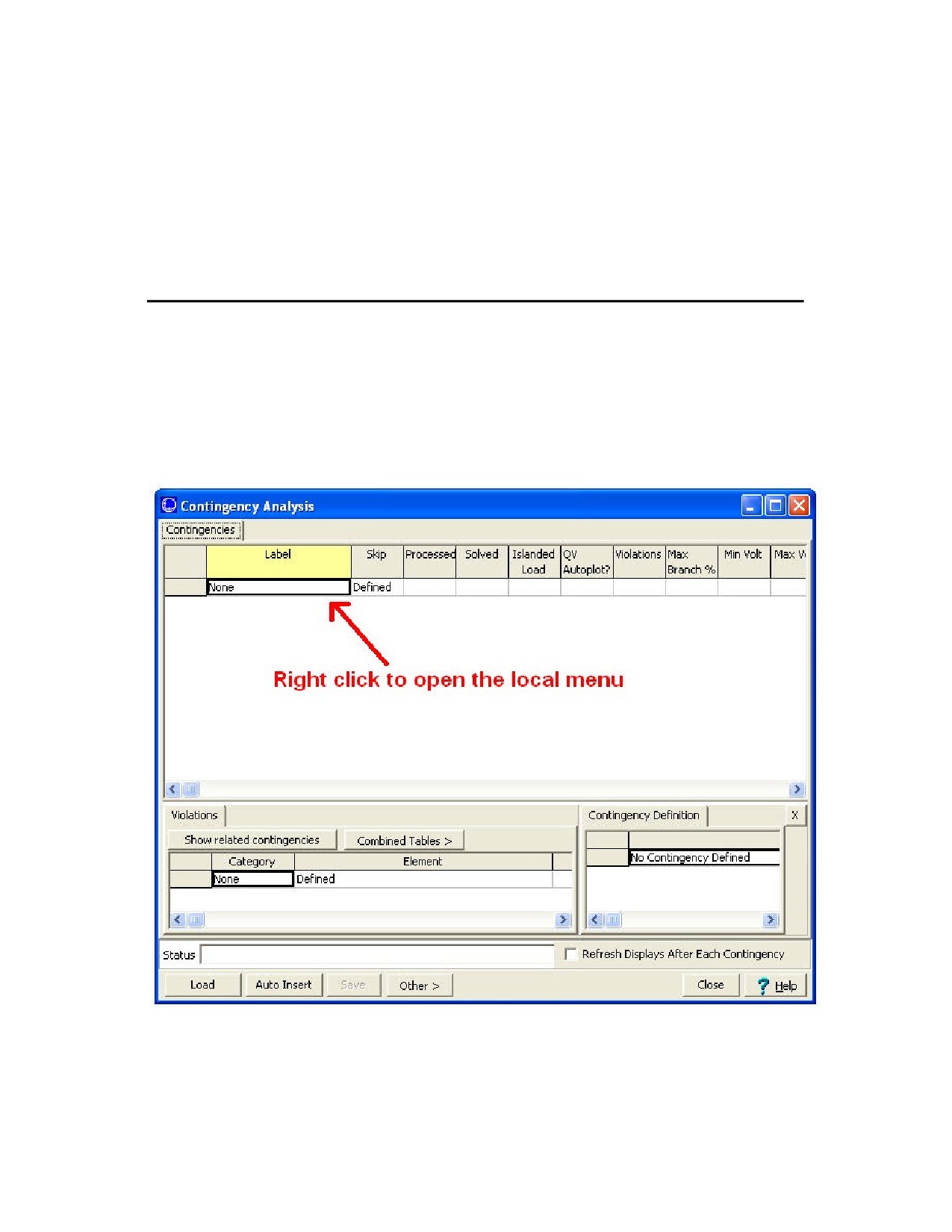
Tutorial: Contingency Analysis

This tutorial will walk you through the basic commands necessary to insert contingencies and hav e Simulator

automatically analyze the results. Please see Introduction to Contingency Analysis for the necessary background

information regarding the capabilities and uses of the Contingency Analysis tool.

For this tutorial, we will use an existing 7-bus case.

· Open case B7SCOPF from the "Program Files/PowerWorld/Simulator/Sample Cases" directory.

· Ensure Simulator is in Run Mode.

· Select Contingency Analysis from the Tools main menu item. Simulator opens the Contingency Analysis Dialog.

Contingency Analysis Dialog

When you access the contingency analysis tool for the first time, no contingencies are defined, so only the

Contingencies tab is visible. Once you have defined contingencies for your case, all four tabs of the contingency

analysis dialog will be visible (Contingencies, Lines/Buses/Interfaces, Options, and Summary).

949

Content      ..     22      23      24